5 Assessing Data Quality

By the end of this chapter you will be able to:

• Apply the TSE framework to identify survey quality issues systematically
• Analyze duration outliers and understand their implications for measurement error
• Conduct sensitivity analysis to test the robustness of filtering decisions
• Use CES quality flags to create a clean analysis sample
• Document analytical decisions for reproducible research
• Understand when quality issues reflect measurement vs. representation errors

The previous chapter established familiarity with CES data structure, variable naming, and label creation. We can load the data and understand what each column represents. Now we assess which responses are trustworthy.

Not all survey responses are equally valid. Some respondents rush through questions without reading carefully. Technical glitches corrupt data. Bots or fraudulent respondents provide nonsense answers. Before exploring substantive patterns, we need systematic quality assessment.

This chapter applies the Total Survey Error framework from Chapter 3 to identify problematic responses using multiple quality indicators. We’ll examine duration outliers, attention checks, duplicate detection, and other signals. The goal: a clean analysis sample that supports credible inference without over-filtering legitimate variation in survey behavior.

5.1 Setting up

import numpy as np
import pandas as pd
import matplotlib.pyplot as plt
from statsmodels.distributions.empirical_distribution import ECDF
from scipy.stats import trim_mean, mstats
import json

data_path = "data/source/ces-2021/2021 Canadian Election Study v2.0.dta"
ces = pd.read_stata(data_path, convert_categoricals=False)
ces.info()

<class 'pandas.core.frame.DataFrame'>
RangeIndex: 20968 entries, 0 to 20967
Columns: 1059 entries, cps21_StartDate to pes21_weight_general_restricted
dtypes: datetime64[ns](7), float32(22), float64(753), int16(2), int32(2), int8(180), object(93)
memory usage: 142.1+ MB

5.2 Design-aware quality assessment

Our aim is to identify clear low-quality responses without over-pruning legitimate variation. In TSE terms, these checks target measurement (e.g., inattention, straightlining) and representation artifacts (e.g., duplicates).

Survey research involves a fundamental tension: we want to remove genuinely problematic data while preserving legitimate diversity in how people engage with surveys. Some respondents are naturally fast readers. Others take longer because they’re thoughtful, not inattentive. The TSE framework helps us think systematically about this challenge.

Rather than applying arbitrary rules (“anyone who completes in under X minutes is bad”), we use the framework to understand what each quality indicator reveals. Duration outliers might signal measurement problems (left tab open) or representation problems (bots). Attention check failures indicate measurement issues. Duplicate IPs suggest representation threats (same person responding twice).

The TSE lens transforms quality assessment from a checklist into principled reasoning: For each indicator, what type of error does it detect? How severe is the threat? What assumptions underlie our filtering decision? This disciplined thinking distinguishes between removing artifacts and inappropriately narrowing our sample to “ideal” respondents who might not represent the population.

We’ll work with duration, attention checks, and duplicate flags, then rely on the CES team’s consolidated cps21_data_quality as our primary gate.

5.3 Mapping quality indicators to TSE framework

Chapter 3 introduced the Total Survey Error framework, which distinguishes between representation errors (who responds) and measurement errors (what they report). Quality assessment operationalizes these concepts using observable indicators.

The CES provides multiple quality flags that map to TSE components:

TSE Component	Quality Issue	CES Indicator	Detection Method
Measurement Error	Inattentive responses	cps21_attention_check	Failed obvious check question
Measurement Error	Straightlining	cps21_inattentive	Identical answers across batteries
Measurement Error	Impossibly fast	cps21_time	Duration < 5 minutes
Measurement Error	Technical artifacts	cps21_time	Duration > 300 minutes
Representation Error	Duplicate responses	cps21_duplicates_pid_flag	Same person ID appears twice
Representation Error	Bot/fraud	cps21_duplicate_ip_demo_flag	Same IP + demographics
Processing Error	Data consolidation	cps21_data_quality	Combines multiple flags

Our workflow examines each indicator, conducts sensitivity analysis to test filtering decisions, and applies a principled quality gate that balances rigor with inclusivity.

Key principle: We’re not seeking perfection (impossible in survey research) but rather identifying clear quality problems while preserving legitimate variation in how people respond to surveys.

5.4 Initial quality diagnostics

The CES includes several data quality indicators that help us assess response quality:

Survey Duration: Respondents who complete the survey too quickly may not have read questions carefully. However, we must be careful not to exclude people who are simply fast readers or familiar with political topics.

Attention Checks: Questions with obvious correct answers help identify inattentive respondents. The CES uses cps21_attention_check where 0 indicates the respondent passed the attention check.

Response Patterns: “Straightlining” (giving the same response to all questions in a battery) or random response patterns may indicate poor data quality.

Completion Status: The final CES dataset includes only respondents who completed the survey. Those with serious data quality issues were removed during cleaning, but some lower-quality responses are flagged with variables like cps21_inattentive, cps21_duplicates_pid_flag, and cps21_duplicate_ip_demo_flag.

)

# Robust attention-check summary (code semantics can vary by survey)
att = ces.get("cps21_attention_check")
if att is not None:
    print("Attention check distribution:")
    print(att.value_counts(dropna=False).sort_index())
else:
    print("No attention check variable found.")

# Duplicates and inattentiveness flags (interpret 1/0 explicitly if known)
for c in ["cps21_inattentive", "cps21_duplicates_pid_flag", "cps21_duplicate_ip_demo_flag"]:
    if c in ces.columns:
        print(f"\n{c}:")
        print(ces[c].value_counts(dropna=False).sort_index())

Attention check distribution:
cps21_attention_check
0.0    20968
Name: count, dtype: int64

cps21_inattentive:
cps21_inattentive
0.0    19115
1.0     1853
Name: count, dtype: int64

cps21_duplicates_pid_flag:
cps21_duplicates_pid_flag
0.0    20876
1.0       92
Name: count, dtype: int64

cps21_duplicate_ip_demo_flag:
cps21_duplicate_ip_demo_flag
0.0    20936
1.0       32
Name: count, dtype: int64

Interpreting Quality Indicators: Artifacts vs. Respondent Behavior

Quality indicators require careful interpretation:

Extreme durations (>300 min): Almost certainly technical artifacts

• Browser tab left open overnight
• Computer sleep/wake cycles
• Time zone miscalculations in logging

Very fast completions (<5 min): Could indicate multiple issues

• Bots or fraudulent responses
• Straightlining (same answer to all questions)
• Genuine fast readers who are familiar with politics

Failed attention checks: Clear measurement problem

• Respondent not reading questions carefully
• Possible language/comprehension barriers

The key distinction: Technical artifacts should be removed (they tell us nothing about respondents). Legitimate variation in response patterns should be preserved (fast readers exist!). Quality assessment walks this line by using multiple indicators rather than single arbitrary cutoffs.

A note on extreme durations: Very long times usually reflect paradata artifacts-tabs left open, laptop sleep, or time-zone parsing-rather than genuine answering behavior. We treat such spikes as artifacts, not respondent traits.

5.5 Analyzing survey duration outliers

5.5.1 Duration distribution and outliers

Survey duration reveals data quality issues. Extremely long durations (>300 minutes) likely reflect technical artifacts-respondents left browser tabs open rather than actively completing questions for five hours. We examine the distribution to identify reasonable exclusion thresholds.

Let’s investigate the duration outliers systematically. First, we’ll get detailed statistics:

dur = ces["cps21_time"].dropna()
duration_stats = dur.describe(percentiles=[.01,.05,.10,.25,.50,.75,.90,.95,.99])
print(duration_stats)

count    20968.000000
mean       145.160446
std       1018.010498
min          6.033333
1%           8.866667
5%          11.283334
10%         12.933333
25%         16.583334
50%         22.083334
75%         31.254167
90%         53.183334
95%        127.452503
99%       3429.498054
max      26252.583984
Name: cps21_time, dtype: float64

print(f"Minimum: {duration_stats['min']:.1f} minutes = {duration_stats['min']/60:.1f} hours")
print(f"Median: {duration_stats['50%']:.1f} minutes = {duration_stats['50%']/60:.1f} hours")
print(f"99th percentile: {duration_stats['99%']:.1f} minutes = {duration_stats['99%']/60:.1f} hours")
print(f"Maximum: {duration_stats['max']:.1f} minutes = {duration_stats['max']/60:.1f} hours")

Minimum: 6.0 minutes = 0.1 hours
Median: 22.1 minutes = 0.4 hours
99th percentile: 3429.5 minutes = 57.2 hours
Maximum: 26252.6 minutes = 437.5 hours

Typical durations:

• The median (50th percentile) is about 22 minutes
• 75% finished in under 31 minutes
• Even the 95th percentile is about 127 minutes (~2 hours)

Outliers:

• The 99th percentile jumps to 3429.5 minutes (~57 hours), which is not realistic for a survey
• The maximum is over 26,000 minutes (~437 hours, or 18 days), which is almost certainly an error (e.g., someone left the survey open)

Interpretation:

• The vast majority of respondents completed the survey in a normal time frame
• A very small number of responses have extremely high durations, which heavily skew the mean (average) and standard deviation
• These outliers should be investigated and likely excluded from analyses that are sensitive to duration

Let’s count some extreme outliers:

for extremity in [1_000, 5_000, 10_000]:
    print(f"N respondents with survey duration > {extremity} minutes: {len(ces[ces['cps21_time'] > extremity])}")

N respondents with survey duration > 1000 minutes: 477
N respondents with survey duration > 5000 minutes: 150
N respondents with survey duration > 10000 minutes: 61

5.5.2 Comparing visualization approaches for duration data

Different visualization techniques reveal different aspects of the duration distribution. Let’s compare several approaches:

# Guard log-transform against non-positive values
dur_pos = dur[dur > 0]
log_duration = np.log10(dur_pos)

# Compare visualizations for outlier-heavy data
fig, axes = plt.subplots(2, 3, figsize=(18, 12))
fig.suptitle('Survey Duration: Visualization Comparisons', y=0.98)

# 1) Full-range histogram (shows compression)
axes[0,0].hist(dur, bins=50, edgecolor='black', alpha=0.7)
axes[0,0].set_title('Histogram (Full Range)\nOutliers compress main mass')
axes[0,0].set_xlabel('Minutes'); axes[0,0].set_ylabel('Count')

# 2) Reasonable cutoff (≤120 min)
cut = 120
dur_cut = dur[dur <= cut]
axes[0,1].hist(dur_cut, bins=30, edgecolor='black', alpha=0.7)
axes[0,1].axvline(dur_cut.median(), color='red', linestyle='--', label=f"Median {dur_cut.median():.1f}")
axes[0,1].legend(); axes[0,1].set_title(f'Histogram (≤{cut} min)')
axes[0,1].set_xlabel('Minutes')

# 3) Box plot (full range)
axes[0,2].boxplot(dur.dropna(), patch_artist=True,
                  boxprops=dict(facecolor='lightblue', alpha=0.7))
axes[0,2].set_title('Box Plot (Full Range)')
axes[0,2].set_ylabel('Minutes'); axes[0,2].set_xticklabels(['Duration'])

# 4) Log10 histogram (positive durations)
axes[1,0].hist(log_duration, bins=40, edgecolor='black', alpha=0.7)
axes[1,0].set_title('Log₁₀(Duration)'); axes[1,0].set_xlabel('log10 minutes')

# 5) ECDF (≤300 min)
dur_300 = dur[dur <= 300]
ecdf = ECDF(dur_300)
axes[1,1].plot(ecdf.x, ecdf.y, marker='.', linestyle='none', alpha=0.7)
axes[1,1].set_title('ECDF (≤300 min)'); axes[1,1].set_xlabel('Minutes'); axes[1,1].set_ylabel('Cum. prob.')

# 6) Violin (≤120 min)
axes[1,2].violinplot([dur_cut], positions=[1], showmeans=True, showmedians=True)
axes[1,2].set_title('Violin (≤120 min)'); axes[1,2].set_ylabel('Minutes'); axes[1,2].set_xticks([1]); axes[1,2].set_xticklabels(['Duration'])

plt.tight_layout(); plt.show()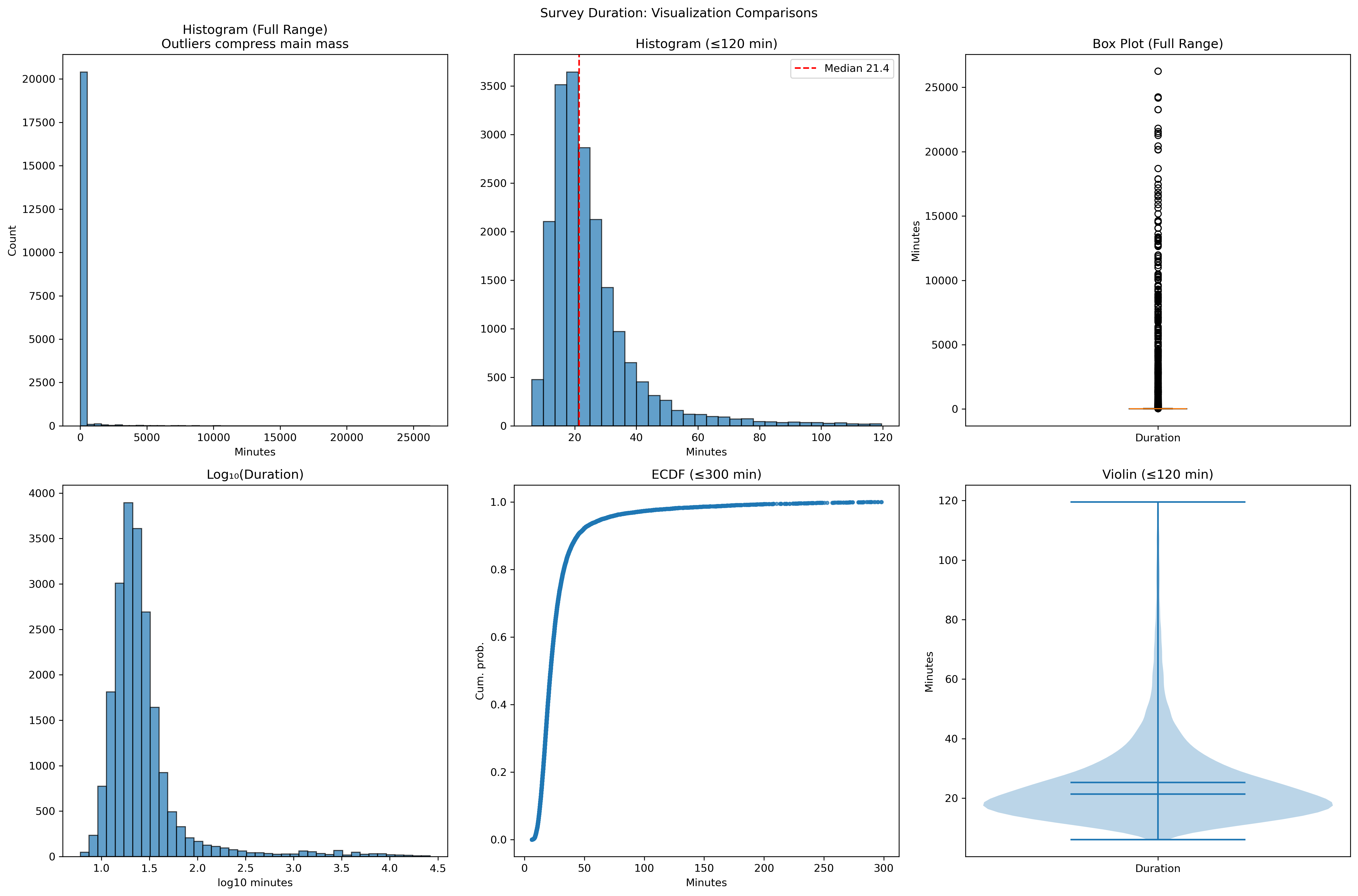

This comparison reveals the trade-offs between different visualization approaches for outlier-heavy data. The key lesson: the same data can look completely different depending on how you visualize it. The full-range histogram hides the main distribution, while the log transformation and ECDF reveal patterns that would otherwise be invisible.

The 99th percentile (3,429 minutes ≈ 57 hours) confirms that extreme values are artifacts. Most respondents complete the survey in 17-31 minutes (interquartile range).

5.6 Sensitivity analysis: Testing filtering decisions

Before proceeding with analysis, it’s crucial to understand how different filtering decisions affect our results. This is an example of sensitivity analysis-testing whether our substantive conclusions change with different reasonable methodological choices.

def summarize_duration(series):
    """Generate comprehensive summary statistics for duration data."""
    x = pd.Series(series).dropna().to_numpy()
    if x.size == 0:
        return {'n':0,'mean':np.nan,'median':np.nan,'IQR':np.nan,'MAD':np.nan,
                'trim_mean_5%':np.nan,'winsor_mean_1%':np.nan}
    q1,q3 = np.quantile(x,[.25,.75]); iqr = q3-q1
    mad = np.median(np.abs(x - np.median(x)))  # Median Absolute Deviation
    return {
        'n': x.size, 'mean': x.mean(), 'median': float(np.median(x)),
        'IQR': iqr, 'MAD': mad,
        'trim_mean_5%': float(trim_mean(x, 0.05)),  # Remove top/bottom 5%
        'winsor_mean_1%': float(mstats.winsorize(x, limits=0.01).mean()),  # Cap extremes
    }

# Compare different filtering strategies
base_n = dur.notna().sum()
approaches = {
    'No filter': dur,
    '5-300 min': dur.where(dur.between(5,300)),
    '≤120 min': dur.where(dur <= 120),
    '5-95%':   dur.where(dur.between(dur.quantile(.05), dur.quantile(.95)))
}
rows=[]
for name, s in approaches.items():
    d = summarize_duration(s)
    d['% excluded'] = round((base_n - d['n'])/base_n*100, 2)
    rows.append(pd.Series(d, name=name))
comparison = pd.DataFrame(rows).round(2)
print("=== Sensitivity to filtering ===")
print(comparison)

=== Sensitivity to filtering ===
                 n    mean  median    IQR   MAD  trim_mean_5%  winsor_mean_1%  \
No filter  20968.0  145.16   22.08  14.67  6.58         26.43           92.53   
5-300 min  20287.0   28.57   21.70  13.53  6.23         24.21           28.08   
≤120 min   19869.0   25.31   21.40  12.78  5.97         23.42           25.20   
5-95%      18881.0   26.42   22.08  12.80  5.85         24.26           26.28   

           % excluded  
No filter        0.00  
5-300 min        3.25  
≤120 min         5.24  
5-95%            9.95  

Key insights from our sensitivity analysis:

1. Robust measures are stable: The median stays around 21-22 minutes regardless of filtering approach
2. Mean is sensitive to outliers: Varies dramatically from 25-145 minutes depending on how we handle extreme values
3. Robust estimators work: Trimmed and winsorized means are much closer to the filtered means than the raw mean
4. Modest exclusions sufficient: Even conservative filtering (5-300 minutes) removes the most problematic cases while retaining 96.7% of responses

This demonstrates why we use robust measures (median, IQR) for describing duration rather than means and standard deviations. The extreme values are artifacts, not information about survey behavior.

Research decision: Conservative filtering (5-300 minutes) removes obvious artifacts while retaining 96.7% of responses. This balances data quality with sample retention.

This analysis demonstrates that our substantive conclusions about “typical” survey completion time (~22 minutes) are robust to different reasonable filtering decisions.

5.7 Building a quality gate

Rather than applying multiple individual filters throughout our analysis, we create a systematic approach to quality filtering. The CES helpfully provides a single quality flag that represents the researchers’ overall assessment.

# Examine the CES data quality flag
quality_flag_counts = ces['cps21_data_quality'].value_counts().sort_index()
print("CES Data Quality Flag Distribution:")
print(quality_flag_counts)
print("\nInterpretation: 0 = high quality, other values = quality issues")

CES Data Quality Flag Distribution:
cps21_data_quality
0.0    19009
1.0       74
2.0       32
4.0     1853
Name: count, dtype: int64

Interpretation: 0 = high quality, other values = quality issues

We’ve done extensive quality diagnostics, but the CES researchers have already provided us with a consolidated quality assessment. We use this as our primary filter while understanding what it represents.

This is design-aware filtering: leverage the research team’s integrated assessments rather than reinventing ad-hoc rules. We remain transparent about what’s being removed.

# Apply quality filtering using the CES data quality flag
ces_clean = ces[ces["cps21_data_quality"] == 0].copy()

print(f"Original sample: {len(ces):,}")
print(f"High-quality responses: {len(ces_clean):,}")
print(f"Retention rate: {len(ces_clean)/len(ces):.1%}")

Original sample: 20,968
High-quality responses: 19,009
Retention rate: 90.7%

# Check if our quality filtering addressed the duration outliers
print("Duration statistics after quality filtering:")
print(ces_clean['cps21_time'].describe())

Duration statistics after quality filtering:
count    19009.000000
mean        23.123240
std          9.800128
min          6.033333
25%         16.066668
50%         20.983334
75%         27.916666
max         59.966667
Name: cps21_time, dtype: float64

Much better! The quality flag has effectively removed the extreme outliers while retaining the vast majority of responses. This is exactly what we want-a principled approach that removes clearly problematic cases without being overly restrictive.

5.8 Documenting the analysis sample

5.8.1 Creating a processing summary

We document our data processing decisions for reproducibility:

# Save our cleaned dataset for future use
process_data = "data/processed/ces2021_cleaned.parquet"
ces_clean.to_parquet(process_data, index=False)

# Document our sample characteristics
sample_summary = {
    "original_n": len(ces),
    "final_n": len(ces_clean),
    "retention_rate": len(ces_clean) / len(ces),
    "mean_age": ces_clean["cps21_age"].mean(),
    "median_duration_minutes": ces_clean["cps21_time"].median(),
}

print("Analysis sample summary:")
for key, value in sample_summary.items():
    if isinstance(value, float):
        print(f"  {key}: {value:.3f}")
    else:
        print(f"  {key}: {value}")

Analysis sample summary:
  original_n: 20968
  final_n: 19009
  retention_rate: 0.907
  mean_age: 51.44652557373047
  median_duration_minutes: 20.983333587646484

5.8.2 Saving provenance metadata

We save both the cleaned CSV and a provenance JSON with the source filename, creation time, and sample counts. Future you will thank present you.

meta = {
    "source_file": data_path,
    "created_utc": pd.Timestamp.utcnow().isoformat(),
    "n_original": int(len(ces)),
    "n_clean": int(len(ces_clean)),
}
with open("data/processed/ces2021_cleaned_meta.json", "w") as f:
    json.dump(meta, f, indent=2)

Future analyses can begin with the cleaned data rather than repeating all the cleaning steps. The provenance file documents our processing decisions.

5.9 Ethical considerations in quality filtering

Quality assessment decisions have ethical dimensions that extend beyond technical correctness. When we exclude responses as “low quality,” we’re making judgments about whose voices count in our analysis.

5.9.1 The responsibility of filtering

Survey respondents have shared their views under specific conditions-informed consent, confidentiality protections, and commitments about how their data will be used. When we filter responses, we must ensure our decisions are:

• Principled: Based on clear criteria linked to data quality, not convenient for our hypotheses
• Transparent: Fully documented so others can evaluate our choices
• Inclusive: Erring toward inclusion when quality indicators are ambiguous
• Design-aware: Respecting the survey team’s expertise rather than inventing ad-hoc rules

5.9.2 Balancing rigor and representation

The tension between data quality and sample representativeness is particularly acute when quality problems correlate with demographic characteristics. For example, if older respondents or those with less formal education are more likely to fail attention checks, aggressive filtering could systematically exclude their perspectives.

This doesn’t mean we accept low-quality data. Rather, it means:

1. Using multiple indicators: No single measure perfectly captures quality
2. Examining patterns: Understanding which groups are disproportionately affected
3. Documenting impact: Reporting how filtering changes sample composition
4. Considering alternatives: Weighting or robustness checks as complements to exclusion

5.9.3 The CES quality flag as ethical anchor

The CES data quality flag represents extensive validation by survey methodologists who understand the tradeoffs. By adopting it as our primary gate, we’re:

• Leveraging expert judgment rather than imposing our own preferences
• Ensuring consistency with how the CES team intended the data to be used
• Maintaining alignment with published CES research for comparability
• Taking responsibility for the filtering choice (it’s our decision to use their flag)

This approach balances methodological rigor with ethical responsibility. We remove clear problems while preserving the diversity of perspectives that makes survey research valuable for understanding public opinion.

5.10 Looking forward: From quality to exploration

This chapter has equipped you with essential skills for transforming raw survey data into trustworthy analysis samples. We’ve learned to:

• Apply systematic quality assessment using multiple indicators from the TSE framework
• Make principled decisions about data filtering using both individual diagnostics and comprehensive quality flags
• Conduct sensitivity analysis to test the robustness of our filtering decisions
• Document all processing steps for reproducible research

5.10.1 Key principles for survey data quality assessment

Design-aware filtering: Use the research team’s documented quality assessments rather than inventing ad-hoc rules. The CES data quality flag consolidates multiple indicators based on extensive validation.

Sensitivity analysis: Test whether key patterns persist across different reasonable analytical choices. Robust findings should not depend on arbitrary decisions about exact cutoff values.

Documentation: Keep detailed records of all processing decisions, including the rationale for filtering criteria and the impact on sample composition.

Principled quality assessment: Use multiple indicators of data quality but avoid being overly restrictive. The goal is to remove clearly problematic cases while preserving legitimate variation in response patterns.

5.10.2 Preparing for exploratory analysis

The cleaned dataset we’ve created provides a solid foundation for exploratory analysis. We’ve established:

• A systematic approach to quality filtering that removes problematic responses while retaining sample diversity
• Clear variable naming conventions and labeling systems that make analysis interpretable
• Comprehensive documentation of all processing decisions for reproducibility
• Understanding of missing value patterns and appropriate handling strategies

In the next chapter, we’ll use these data to explore political attitudes and behaviors while learning to think carefully about what survey data can and cannot tell us about the broader Canadian population. We’ll examine univariate distributions, explore bivariate relationships, and begin to understand the crucial distinction between describing our sample and making inferences about the population.

5.10.3 Reproducible workflow benefits

The systematic approach we’ve developed provides several important advantages:

Reproducibility: Your analysis can be replicated by others or by yourself at a later date by following the documented processing steps.

Robustness checking: You can easily test whether your results depend on specific analytical choices by modifying filtering criteria and re-running the analysis. The kind of sensitivity analysis we’ve done here becomes straightforward to implement.

Cumulative science: Clear documentation allows future researchers to build on your work rather than starting from scratch. This includes yourself when you return to the analysis months later.

Quality assurance: Systematic quality checks help identify potential problems before they affect substantive conclusions.

5.10.4 Essential takeaways

Survey data processing requires balancing scientific rigor with practical constraints. We want to remove clearly problematic responses without being so restrictive that we bias our sample toward particular types of respondents.

Multiple quality indicators provide more robust assessment than any single criterion. Duration, attention checks, duplicate detection, and response patterns each capture different aspects of data quality.

Sensitivity analysis is crucial for establishing the robustness of analytical decisions. If key patterns disappear with small changes in filtering criteria, they may not be reliable.

Comprehensive documentation enables reproducible research. Every decision should be documented with clear rationale and impact assessment.

Understanding the survey design helps interpret data quality patterns. The Total Survey Error framework provides a systematic way to think about potential problems and appropriate responses.

You now have a trustworthy analysis sample with quality gates and documented provenance. In the next chapter we’ll conduct exploratory data analysis: univariate distributions, bivariate relationships, and design-aware interpretation. We will keep the sample vs. population distinction front and center and introduce weights when we want to speak about Canadians rather than just our respondents.