import numpy as np
import pandas as pd
import matplotlib.pyplot as plt
import seaborn as sns
from statsmodels.distributions.empirical_distribution import ECDF

plt.style.use("qmcp.mplstyle")

ces_clean = pd.read_parquet("data/processed/ces2021_cleaned.parquet")
ces_clean = ces_clean.convert_dtypes()By the end of this chapter you will be able to:
- Conduct univariate exploratory data analysis of survey variables
- Create effective visualizations for both continuous and categorical variables
- Perform bivariate analysis to explore relationships between variables
- Understand the distinction between sample description and population inference
- Apply basic concepts of survey weighting and when to use them
- Interpret survey results with appropriate caution about causal claims
- Document exploratory findings as foundation for theoretical analysis
With a clean, well-documented analysis sample in hand, we can now begin exploring patterns in the data. This chapter focuses on exploratory data analysis (EDA)—the systematic examination of variables and relationships that forms the foundation for more sophisticated theoretical analyses.
This chapter focuses on the Explore stage of our research workflow (?sec-workflow). Exploratory data analysis isn’t optional—it’s essential for understanding data quality, identifying patterns that warrant further investigation, and detecting potential problems before formal hypothesis testing. The time invested in thorough exploration pays dividends in more robust, credible analyses downstream.
Crucially, we’ll learn to think carefully about what our analyses represent. Are we describing our sample, or making claims about the Canadian population? When should we use survey weights, and when is unweighted analysis appropriate? How do we avoid overinterpreting correlational patterns as causal relationships? These distinctions become essential as we move toward the theoretical analyses in ?sec-regression, ?sec-logistic-regression, and ?sec-glms-counts, where we’ll use survey data to test competing theories about political attitudes, ideological constraint, and affective polarization.
6.1 Setting Up for Exploratory Analysis
# Load label mappings from metadata module
# Note: In production, these would be loaded from a YAML file or dedicated module
# For pedagogical clarity, we define them here but acknowledge this should be
# stored separately for maintainability
education_labels = {
    1: "No schooling",
    2: "Some elementary school",
    3: "Elementary school completed",
    4: "Some secondary school",
    5: "Secondary school completed",
    6: "Some technical/community college",
    7: "Technical/community college completed",
    8: "Some university",
    9: "Bachelor's degree",
    10: "Master's degree",
    11: "Professional degree",
    12: "Doctoral degree",
}

party_labels = {
    1: "Liberal",
    2: "Conservative",
    3: "NDP",
    4: "Bloc Québécois",
    5: "Green",
    6: "Other party",
    7: "None of these",
    8: "Don't know/Prefer not to answer",
}

ces_clean = ces_clean.assign(
    education_labeled=ces_clean["cps21_education"].map(education_labels),
    party_id_labeled=ces_clean["cps21_fed_id"].map(party_labels),
)

print(f"Analysis sample: {len(ces_clean):,} respondents")
Analysis sample: 19,009 respondents6.2 Sample vs. Population: A Crucial Distinction
Before we begin exploring our data, we must address a crucial methodological point that affects how we interpret our results. Throughout this chapter, we’ll be analyzing the raw, unweighted survey sample, not the Canadian population. This distinction is fundamental to responsible survey analysis.
Our analysis sample consists of approximately 20,000 Canadians who completed the CES survey. While this is a large and carefully designed sample, it does not perfectly mirror the Canadian population. The CES includes deliberate oversamples of certain groups, such as residents of smaller provinces, to ensure sufficient representation for regional analysis. Not all types of people respond to surveys at equal rates. Younger, less educated, and politically disengaged Canadians are typically harder to reach and less likely to participate. These design features and response patterns mean that our sample proportions do not directly translate to population estimates.
When is unweighted sample analysis appropriate? We use unweighted data when exploring data quality and response patterns, when understanding how survey variables relate to each other conceptually, when developing theoretical insights about political attitudes, and when testing whether measurement approaches work as intended. These are all questions about the structure of political attitudes and the quality of our measures, not about precise population proportions.
What can we not claim from unweighted analysis? We cannot say that sample percentages represent population percentages, that our findings generalize to all Canadians, or that relationships we observe reflect “true” population relationships with known precision. Regional, age, or education distributions in our sample may not match Canadian census data. Political preferences may be biased toward more politically engaged respondents who are more willing to spend time on surveys.
Our goals for exploratory analysis are therefore specific and limited. We want to assess data quality by identifying obvious problems with missing data, outliers, or inconsistent responses. We aim to understand sample composition by learning who participated in this survey and how that might affect our substantive conclusions. We seek to identify patterns for investigation, highlighting relationships that deserve further analysis with proper weights and statistical inference. We also check for bias indicators by looking for patterns suggesting certain groups are over- or underrepresented relative to population benchmarks.
This distinction will become crucial as we progress through the chapter. For now, we’re in “sample exploration” mode, learning about our data to prepare for more sophisticated analysis. Later chapters will introduce survey weights and design-based inference when we want to make claims about the broader Canadian population.
6.3 Understanding Our Sample Demographics
With our clean dataset, we can begin exploring the characteristics of our respondents. This serves two purposes: understanding who participated in the survey, which matters for generalizability, and learning fundamental EDA techniques that apply across many research contexts.
Univariate analysis examines single variables in isolation. For categorical variables like party identification or education level, we create frequency tables and bar charts. For continuous variables like age or income, we examine distributions using histograms and summary statistics. This provides a baseline understanding of each variable before we move to bivariate analysis, which looks at relationships between two variables.
The distinction between univariate and bivariate analysis is straightforward. When we ask “How old are our survey respondents?” or “What percentage support each political party?” we’re conducting univariate analysis, looking at one variable by itself. When we ask “Do older people prefer different parties than younger people?” or “Is education related to income?” we’re conducting bivariate analysis, exploring how variables relate to each other. We start with univariate analysis to understand each variable individually, then move to bivariate analysis to explore relationships.
The choice of descriptive statistics depends on the variable’s measurement scale (?sec-measurement-scales). For nominal data (categories with no order), only frequency counts and mode make sense. For ordinal data (ordered categories), the median is appropriate as it doesn’t assume equal spacing between categories. For interval and ratio scales (continuous measurements), the mean is valid because it treats differences between values as meaningful. Understanding these constraints prevents statistical misuse and guides appropriate analysis choices.
6.3.1 Continuous Variables: Age Distribution
fig, ax = plt.subplots(figsize=(10, 6))
ax.hist(ces_clean["cps21_age"], bins=20, edgecolor="black", alpha=0.7)
ax.set_title("Age Distribution in the Unweighted CES Sample")
ax.set_xlabel("Age")
ax.set_ylabel("Frequency")
ax.axvline(
    ces_clean["cps21_age"].mean(),
    color="red",
    linestyle="--",
    linewidth=2.5,
    label=f'Mean: {ces_clean["cps21_age"].mean():.1f}',
)
ax.legend()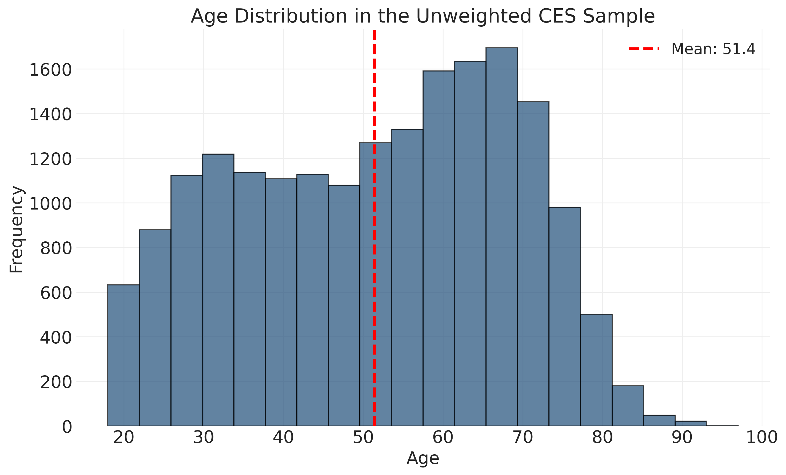
The distribution shows fairly even representation across ages 30-70, with fewer very young and very old respondents. This is typical of telephone and online surveys, which tend to under-represent the youngest adults (busy with education and early careers) and oldest adults (less comfortable with technology or harder to reach).
# Age summary statistics
age_summary = ces_clean['cps21_age'].describe()
summary_report = f"""
Age Distribution Summary:
  Mean: {age_summary['mean']:.1f} years
  Median: {age_summary['50%']:.1f} years
  Range: {age_summary['min']:.0f} to {age_summary['max']:.0f} years
  Standard deviation: {age_summary['std']:.1f} years
"""
print(summary_report)
Age Distribution Summary:
  Mean: 51.4 years
  Median: 53.0 years
  Range: 18 to 97 years
  Standard deviation: 17.2 years
6.3.2 Categorical Variables: Education and Party ID
# Education distribution (categorical variable, mapped to labels) - horizontal bar chart
education_counts = ces_clean['cps21_education'].map(education_labels).value_counts(ascending=False)
fig, ax = plt.subplots(figsize=(12, 6))
ax.barh(range(len(education_counts)), education_counts.values, edgecolor='black', alpha=0.7)
ax.set_title('Education Distribution in the Unweighted CES Sample')
ax.set_ylabel('')
ax.set_xlabel('Frequency')
ax.set_yticks(range(len(education_counts)))
ax.set_yticklabels(education_counts.index)
ax.xaxis.set_major_formatter(plt.matplotlib.ticker.FuncFormatter(lambda x, _: f"{int(x):,}"))
ax.invert_yaxis()
plt.show()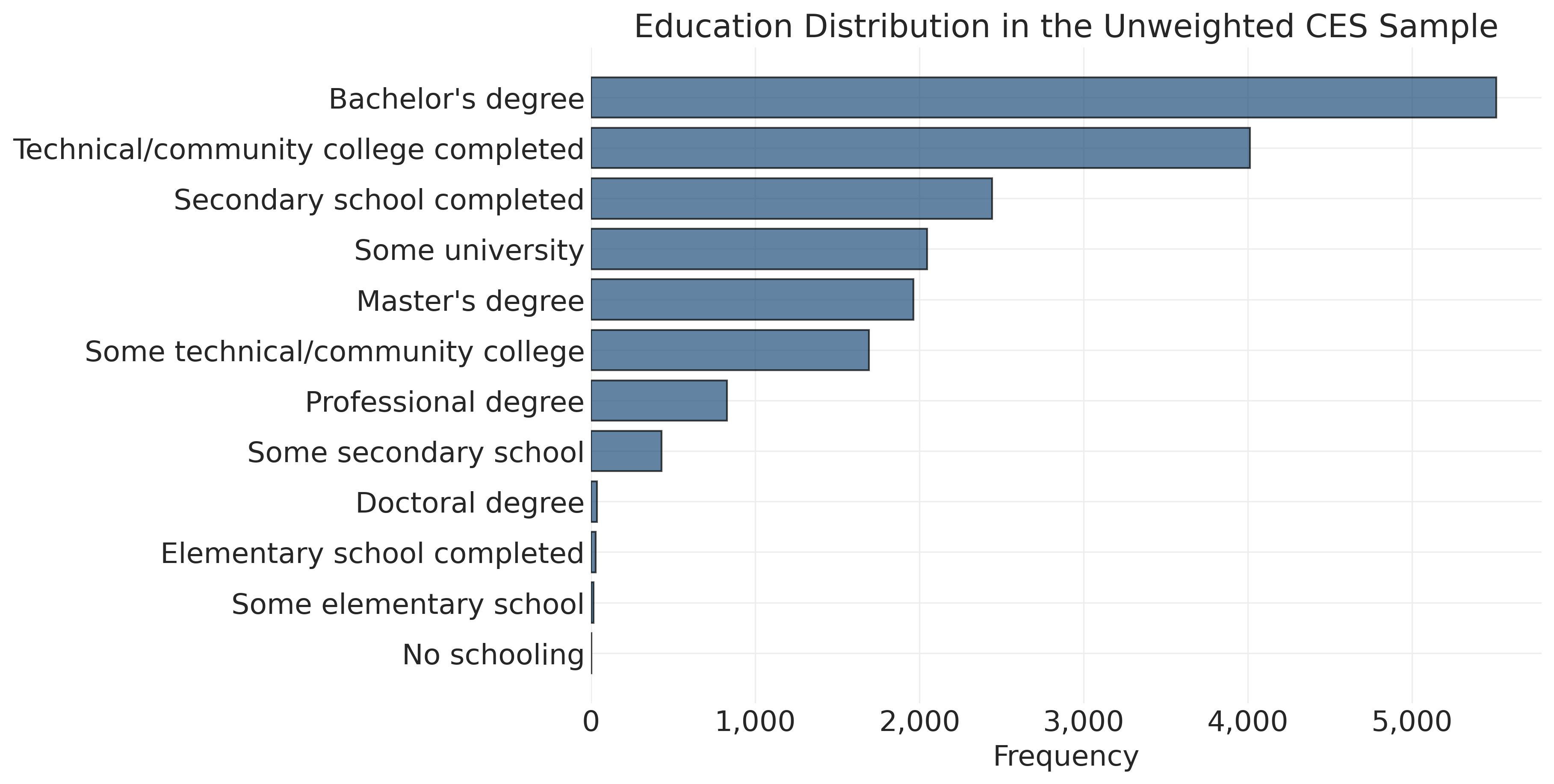
# Party identification patterns
party_counts = ces_clean["party_id_labeled"].value_counts(dropna=False)
party_counts
party_id_labeled
Liberal 5816
Conservative 4376
NDP 2811
None of these 1930
Bloc Québécois 1639
Don't know/Prefer not to answer 1527
Green 504
Other party 406
Name: count, dtype: int64These raw counts show the distribution of party identification in our sample. To understand what these numbers mean and how they were collected, we consult the CES codebook, which provides several crucial pieces of information: the exact question wording read to respondents, the available response options and their numeric codes, how non-responses are handled (Don’t know = -8, Refused = -9, etc.), and any filter conditions that determined which respondents were asked which questions. Understanding these details is essential because apparently similar questions may be worded differently across surveys or over time, affecting how we interpret results.
6.3.3 Variable Families and Question Batteries
Survey questionnaires are organized around theoretical concepts, creating families of related variables. In the CES, major variable families include demographics (age, gender, education, income, region, urban/rural status, language, immigration status), political attitudes (left-right self-placement, issue positions, government evaluation), party evaluations (feeling thermometers, leader ratings, vote choice), political engagement (media consumption, campaign participation), social identities (religious affiliation, union membership, ethnic identification), and data quality indicators (completion time, attention checks, quality flags).
With 400+ variables in the CES, we need systematic approaches to find related variables. Let’s explore some key political attitude variables:
# Examine left-right ideology variable
print("Left-right self-placement variable examination:")
print(f"Variable: cps21_lr_scale_bef_1")
print(f"Total responses: {ces_clean['cps21_lr_scale_bef_1'].count():,}")
print(f"Missing values: {ces_clean['cps21_lr_scale_bef_1'].isna().sum():,}")

# Look at the actual values to identify missing value codes
print(f"\nValue distribution (including missing codes):")
value_counts = ces_clean['cps21_lr_scale_bef_1'].value_counts(dropna=False).sort_index()
for value, count in value_counts.items():
    print(f"  {value}: {count:,}")
Left-right self-placement variable examination:
Variable: cps21_lr_scale_bef_1
Total responses: 19,009
Missing values: 0
Value distribution (including missing codes):
-99: 2,597
0: 481
1: 573
2: 1,312
3: 1,912
4: 1,971
5: 3,079
6: 2,262
7: 2,172
8: 1,502
9: 564
10: 584# Filter out missing values (-99, -88, etc.) to get valid responses
valid_lr = ces_clean["cps21_lr_scale_bef_1"][ces_clean["cps21_lr_scale_bef_1"] >= 0]
valid_lr = valid_lr[valid_lr <= 10] # 0-10 scale
fig, ax = plt.subplots(figsize=(8, 5))
ax.hist(valid_lr, bins=11, edgecolor="black", alpha=0.7)
ax.set_xlabel("Left ← → Right Self-Placement\n0=Left, 10=Right")
ax.set_ylabel("Frequency")
ax.set_title(
"Left → Right Self-Placement Distribution\nUnweighted Sample, Valid Responses Only"
)
from matplotlib.ticker import FuncFormatter
ax.yaxis.set_major_formatter(FuncFormatter(lambda x, _: f"{int(x):,}"))
plt.show()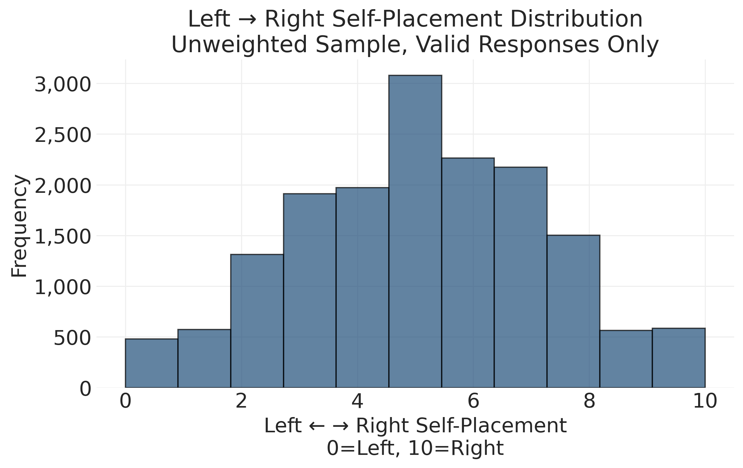
# Calculate response rate for this question
response_rate = (len(valid_lr) / len(ces_clean)) * 100
response_summary = f"""
Response Rate Analysis:
  Valid responses: {len(valid_lr):,}
  Total sample: {len(ces_clean):,}
  Response rate: {response_rate:.1f}%
"""
print(response_summary)
Response Rate Analysis:
  Valid responses: 16,412
  Total sample: 19,009
  Response rate: 86.3%
Political attitude questions often have substantial missing data for several reasons. Many people genuinely don’t have opinions on complex political issues, leading to “Don’t know” responses. Some respondents prefer not to reveal political views and refuse to answer. Abstract concepts like left-right ideology can be difficult to understand, especially for those with limited political interest. Survey fatigue also plays a role, as political batteries often come late in surveys when attention wanes.
These patterns have important implications for analysis. We should always report response rates for political variables and consider whether missing data patterns relate to other variables like education or political interest. We must be cautious about generalizing from smaller valid-response samples, as missing data may not be “missing at random.” If politically sophisticated respondents are more likely to answer ideology questions, patterns we observe may not generalize to the full population. Systematic non-response can bias results in ways that are difficult to detect or correct.
6.4 Bivariate Analysis: Examining Relationships
6.4.1 Cross-Tabulation: Education by Region
Cross-tabulation examines relationships between categorical variables by creating contingency tables. This answers questions like “Does education level vary by region?” or “Are men and women equally likely to support different parties?” A cross-tabulation, or crosstab, creates a table showing how two categorical variables relate. For example, we might show party support within each province, revealing that Quebec strongly favors Liberals while Alberta strongly favors Conservatives, with NDP support remaining similar across provinces. Cross-tabs reveal whether patterns differ across groups, but we must always pay attention to whether percentages are calculated within rows, within columns, or as a percentage of the total.
For this analysis, we’ll use the actual CES region variable to explore how education patterns vary across Canada:
# Cross-tabulation: Education by region using actual CES data
# Note: Using a subset of education categories for readability
education_subset = ces_clean[
    ces_clean["cps21_education"].isin([5, 7, 9, 10, 11])
]  # Key categories
edu_region_crosstab = (
    pd.crosstab(
        education_subset["Region"],
        education_subset["cps21_education"].map(education_labels),
        normalize="index",
    )
    * 100
)  # Convert to percentages


# Education distribution by region (% within each region
# Transposed for readability
edu_region_crosstab_t = edu_region_crosstab.round(1).T
edu_region_crosstab_t.index.name = None
edu_region_crosstab_t.columns.name = None
edu_region_crosstab_t| Atlantic | Ontario | Quebec | Territories | West | |
|---|---|---|---|---|---|
| Bachelor's degree | 31.6 | 40.2 | 34.2 | 41.2 | 38.2 |
| Master's degree | 10.5 | 13.6 | 14.4 | 29.4 | 12.3 |
| Professional degree | 4.2 | 6.3 | 5.1 | 2.9 | 5.5 |
| Secondary school completed | 19.7 | 14.1 | 19.4 | 5.9 | 16.3 |
| Technical/community college completed | 34.0 | 25.9 | 26.9 | 20.6 | 27.7 |
# Visualize the cross-tabulation: grouped bar chart
fig, ax = plt.subplots(figsize=(16, 8))

# Position bars: one group per region
x_pos = np.arange(len(edu_region_crosstab.index))

# Calculate bar width: divide available space by number of education levels
width = 0.8 / len(edu_region_crosstab.columns)

# Create one set of bars for each education level
for i, edu_level in enumerate(edu_region_crosstab.columns):
    # Offset each education level's bars slightly
    ax.bar(x_pos + i * width, edu_region_crosstab[edu_level],
           width, label=edu_level, alpha=0.8)

ax.set_title('Education Distribution by Region (Unweighted Sample)')
ax.set_xlabel('')
ax.set_ylabel('Percentage within Region')

# Center tick labels under each group of bars
ax.set_xticks(x_pos + width * (len(edu_region_crosstab.columns) - 1) / 2)
ax.set_xticklabels(edu_region_crosstab.index, ha='right')

# Place legend below chart to avoid covering data
ax.legend(title='', bbox_to_anchor=(0.5, -0.15), loc='upper center',
          frameon=False, ncol=4)
plt.tight_layout()
plt.show()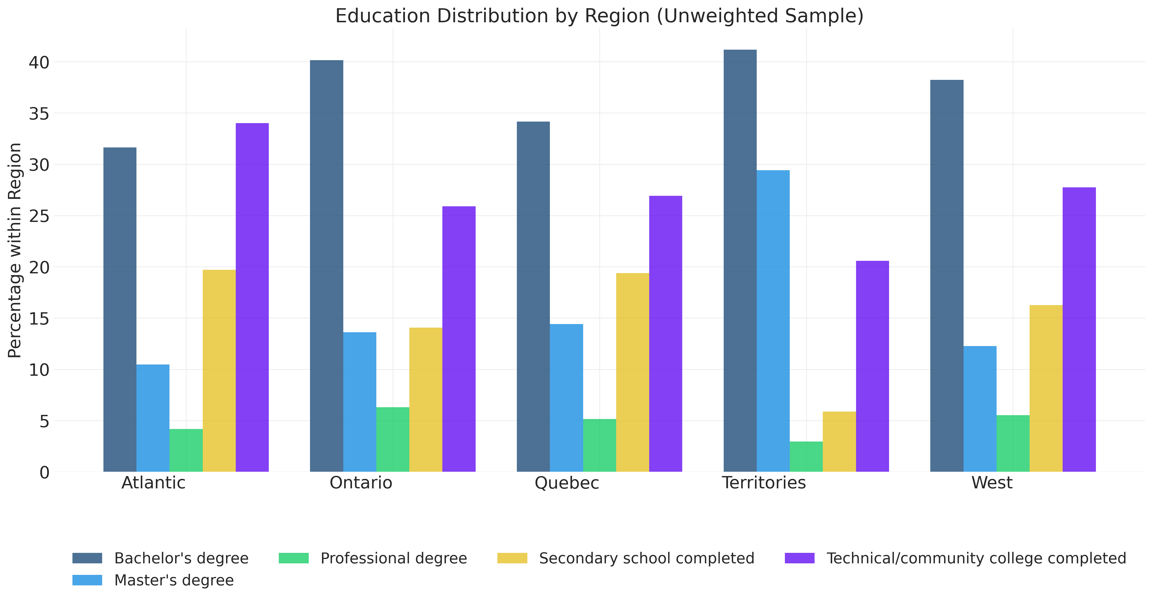
6.4.2 Continuous by Continuous: Age and Political Ideology
Correlation measures linear relationships between continuous variables. Let’s explore the relationship between age and left-right self-placement. Correlation tells us if two continuous variables tend to increase or decrease together. A correlation of +1 indicates a perfect positive relationship where as one variable increases, the other always increases by a predictable amount. Height and weight, for example, often correlate around +0.7. A correlation of 0 indicates no linear relationship, meaning knowing one variable tells you nothing about the other. Shoe size and political preference would fall into this category. A correlation of -1 indicates a perfect negative relationship where as one variable increases, the other always decreases. Hours of TV watching and hours of reading might correlate around -0.3.
Correlation and the Mathematics of Linear Relationships
Pearson’s correlation coefficient (r) measures the strength and direction of linear relationships between two continuous variables. It is calculated as:
\[r = \frac{\sum (x_i - \bar{x})(y_i - \bar{y})}{\sqrt{\sum (x_i - \bar{x})^2 \sum (y_i - \bar{y})^2}}\]
This formula captures how much variables co-vary (numerator) relative to how much they vary individually (denominator). The result is always between -1 and +1:
- r = +1: Perfect positive linear relationship (all points on upward-sloping line)
- r = 0: No linear relationship (knowing X tells you nothing about Y)
- r = -1: Perfect negative linear relationship (all points on downward-sloping line)
Interpreting correlation strength depends on arbitrary conventions like:
- |r| < 0.3: Weak relationship
- 0.3 ≤ |r| < 0.7: Moderate relationship
- |r| ≥ 0.7: Strong relationship
Correlation only measures linear relationships. Variables can have strong nonlinear relationships (e.g., U-shaped) while having r ≈ 0. Always visualize before summarizing.
r² (coefficient of determination) tells you the proportion of variance in one variable explained by the other. For our age-ideology correlation of r = 0.122, r² = 0.015 means age explains only 1.5% of the variation in political ideology.
The crucial point is that correlation does not equal causation. Just because two variables move together doesn’t mean one causes the other. There may be third variables that explain both, or the relationship may be coincidental.
# Correlation between age and left-right self-placement
# Filter out missing values for correlation
valid_lr_data = ces_clean[(ces_clean['cps21_lr_scale_bef_1'] >= 0) &
                          (ces_clean['cps21_lr_scale_bef_1'] <= 10)]

correlation = valid_lr_data['cps21_age'].corr(valid_lr_data['cps21_lr_scale_bef_1'])
print(f"Correlation between age and left-right self-placement: {correlation:.3f}")
Correlation between age and left-right self-placement: 0.122# Create scatter plot
fig, ax = plt.subplots(figsize=(10, 6))
# Add jitter: small random noise to reduce overplotting
# (Many people have same age/ideology, so points stack on top of each other)
age_jitter = valid_lr_data['cps21_age'] + np.random.normal(0, 0.3, len(valid_lr_data))
lr_jitter = valid_lr_data['cps21_lr_scale_bef_1'] + np.random.normal(0, 0.1, len(valid_lr_data))
ax.scatter(age_jitter, lr_jitter, alpha=0.3, s=20)
ax.set_xlabel('Age')
ax.set_ylabel('Left-Right Self-Placement (0=Left, 10=Right)')
ax.set_title(f'Age vs. Left-Right Self-Placement (r = {correlation:.3f})')
ax.set_ylim(-0.5, 10.5)
# Add a trend line
z = np.polyfit(valid_lr_data['cps21_age'], valid_lr_data['cps21_lr_scale_bef_1'], 1)
p = np.poly1d(z)
ax.plot(valid_lr_data['cps21_age'], p(valid_lr_data['cps21_age']), "r--", alpha=0.8)
plt.show()
print(f"Sample size for correlation: {len(valid_lr_data):,}")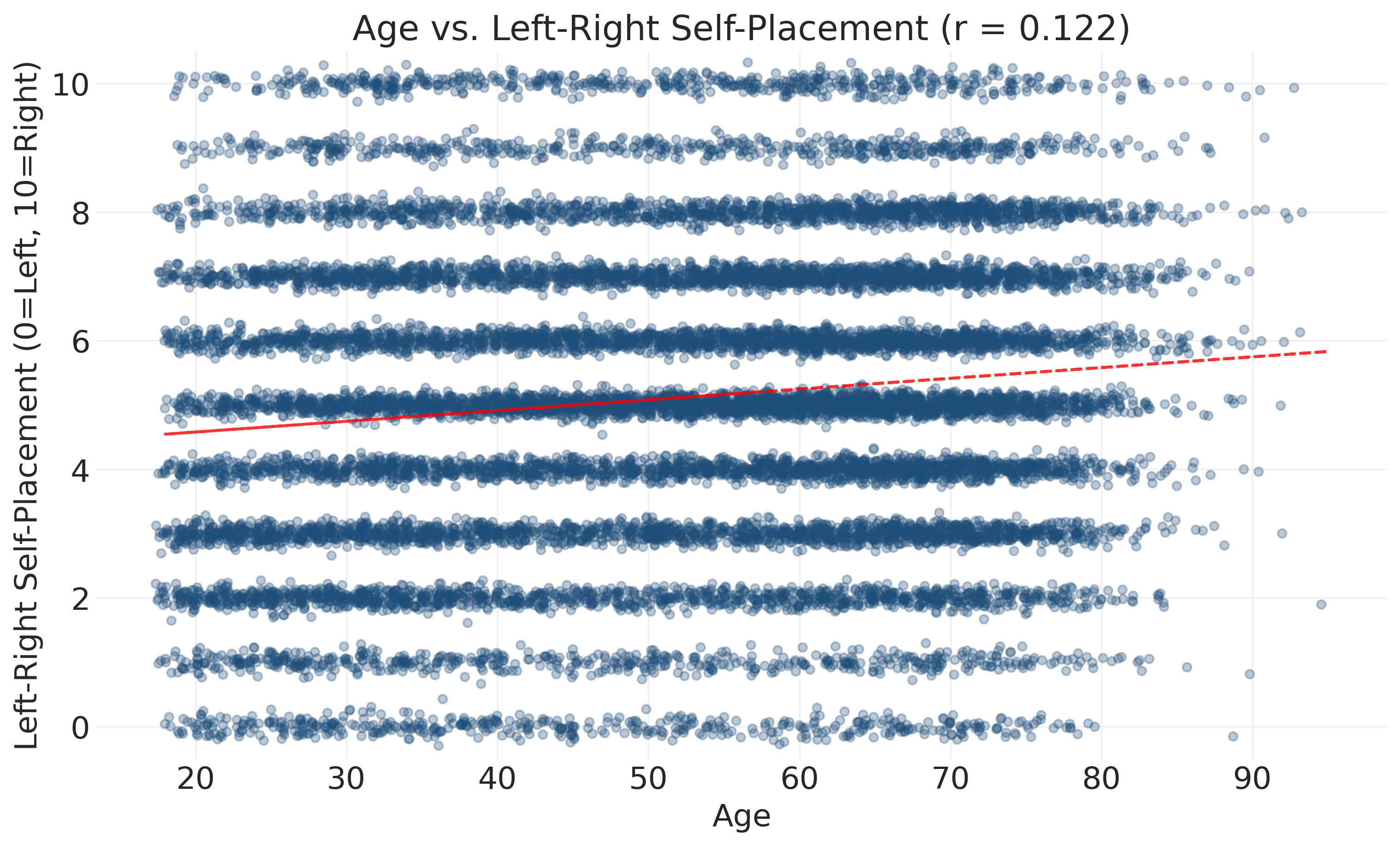
Sample size for correlation: 16,412Interpreting the correlation: The correlation coefficient of r = 0.122 tells us there is a weak positive relationship between age and political ideology in this sample. This means that as age increases, left-right self-placement tends to increase slightly (older people place themselves slightly more to the right), but the relationship is very weak.
Understanding correlation strength: Correlation coefficients range from -1 to +1. Values near 0 indicate weak relationships, while values near -1 or +1 indicate strong relationships. Our r = 0.122 is close to zero, meaning age and ideology are only weakly related in this sample and with this simple model. To understand how much age accounts for ideology, we square the correlation: r² = (0.122)² = 0.015, or about 1.5%. In other words, age only accounts for 1.5% of the variation in political ideology; the other 98.5% is accounted for by other factors (education, income, life experiences, values, etc.).
I’ve used the phrase accounts for here, but I could have also said something like “age explains 1.5% of the variance in ideology in this sample.” When you see it in this kind of context, “explain” is being used as a shorthand for mathematical decomposition of variance; it’s not an explanation in the substantive or theoretical sense.
What this tells us about the data: With 16,000+ respondents, we can be reasonably confident that this weak positive relationship exists in our sample. However, it’s not practically meaningful for understanding individual political attitudes. Knowing someone’s age tells you almost nothing about where they’ll place themselves politically. A 25-year-old and a 75-year-old are nearly as likely to have the same ideology score as different ones. Look at the plot: the red trend line rises only slightly from left to right, while the dominant pattern is the massive scatter of points covering the entire range of ideology scores at every age. Most of the action is in that scatter, not the subtle trend.
Visualization challenges: Beyond the weak correlation, this scatter plot has overplotting issues that make it hard to see patterns. Thousands of respondents have the same age-ideology combinations, causing points to stack on top of each other. The jitter helps somewhat, but we need better visualization approaches to understand the data distribution:
Looking Ahead: From Correlation to Regression
Correlation measures the strength of linear relationships between variables, but it treats both variables symmetrically, meaing neither is the “outcome” we’re trying to predict or explain. In ?sec-regression, we’ll extend these ideas to regression models that distinguish between predictors and outcomes, allow us to make predictions while adjusting for multiple variables simultaneously. We’ll maintain an emphasis on data description and a probabilistic perspective concerned with quantifying uncertainty rather than rigid hypothesis testing.
6.4.3 Alternative Visualization Approaches
# Alternative visualization 1: Hexbin plot (shows density of points)
fig, ax = plt.subplots(figsize=(10, 6))
hb = ax.hexbin(
    valid_lr_data["cps21_age"],
    valid_lr_data["cps21_lr_scale_bef_1"],
    gridsize=30,
    mincnt=1,
    cmap="Blues",
)
ax.set_xlabel("Age")
ax.set_ylabel("Left-Right Self-Placement (0=Left, 10=Right)")
ax.set_title("Age vs. Left-Right Self-Placement (Density Plot)")
cb = fig.colorbar(hb, ax=ax)
cb.set_label("Number of respondents")
plt.show()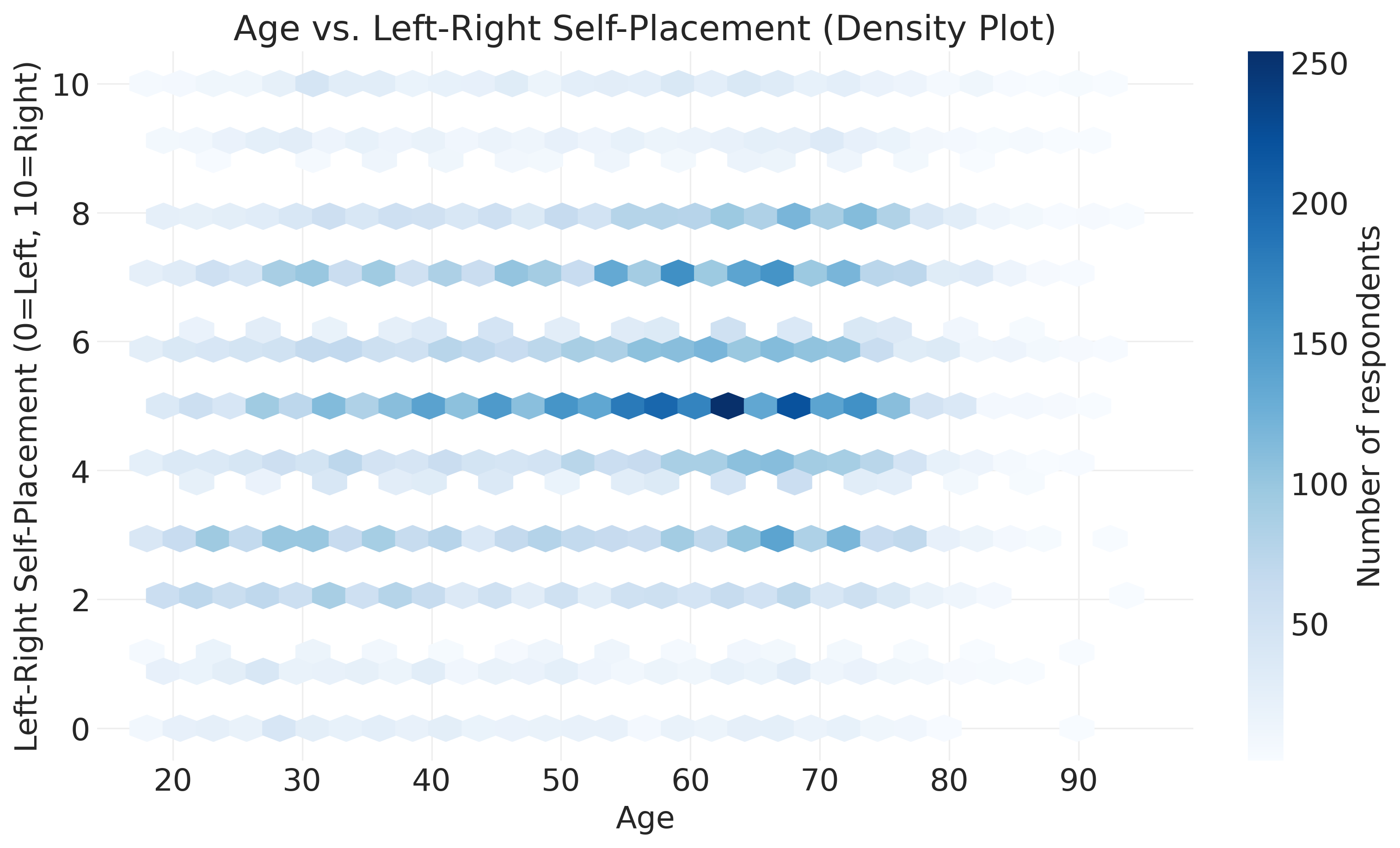
Hexbin plots solve the overplotting problem by dividing the plot area into hexagonal bins and coloring each bin based on how many data points fall into it. Dark blue hexagons indicate many respondents have this combination of age and ideology, light blue hexagons indicate fewer respondents, and white areas indicate no respondents or very few. This lets you see patterns that are invisible in scatter plots. You can identify the most common combinations and spot whether certain age-ideology pairs are unusually rare or common.
# Alternative visualization 2: Horizontal boxplot of ideology by age group
# Create age groups (decades)
age_bins = [18, 29, 39, 49, 59, 69, 79, 100]
age_labels = ["18-28", "29-38", "39-48", "49-58", "59-68", "69-78", "79+"]

# Create a working copy with age groups
lr_by_age = valid_lr_data.copy()
lr_by_age["age_group"] = pd.cut(
    lr_by_age["cps21_age"], bins=age_bins, labels=age_labels, right=False
)

# Check group sizes
print("Sample sizes by age group:")
print(lr_by_age["age_group"].value_counts().sort_index())

fig, ax = plt.subplots(figsize=(10, 8))
sns.boxplot(
    data=lr_by_age, y="age_group", x="cps21_lr_scale_bef_1",
    ax=ax, palette="Set2", order=age_labels
)

ax.set_xlabel("Left-Right Self-Placement (0=Left, 10=Right)")
ax.set_ylabel("Age Group")
ax.set_title("Left-Right Self-Placement by Age Group (Unweighted Sample)")

plt.tight_layout()
plt.show()
Sample sizes by age group:
age_group
18-28 1907
29-38 2444
39-48 2352
49-58 2764
59-68 3683
69-78 2747
79+ 515
Name: count, dtype: int64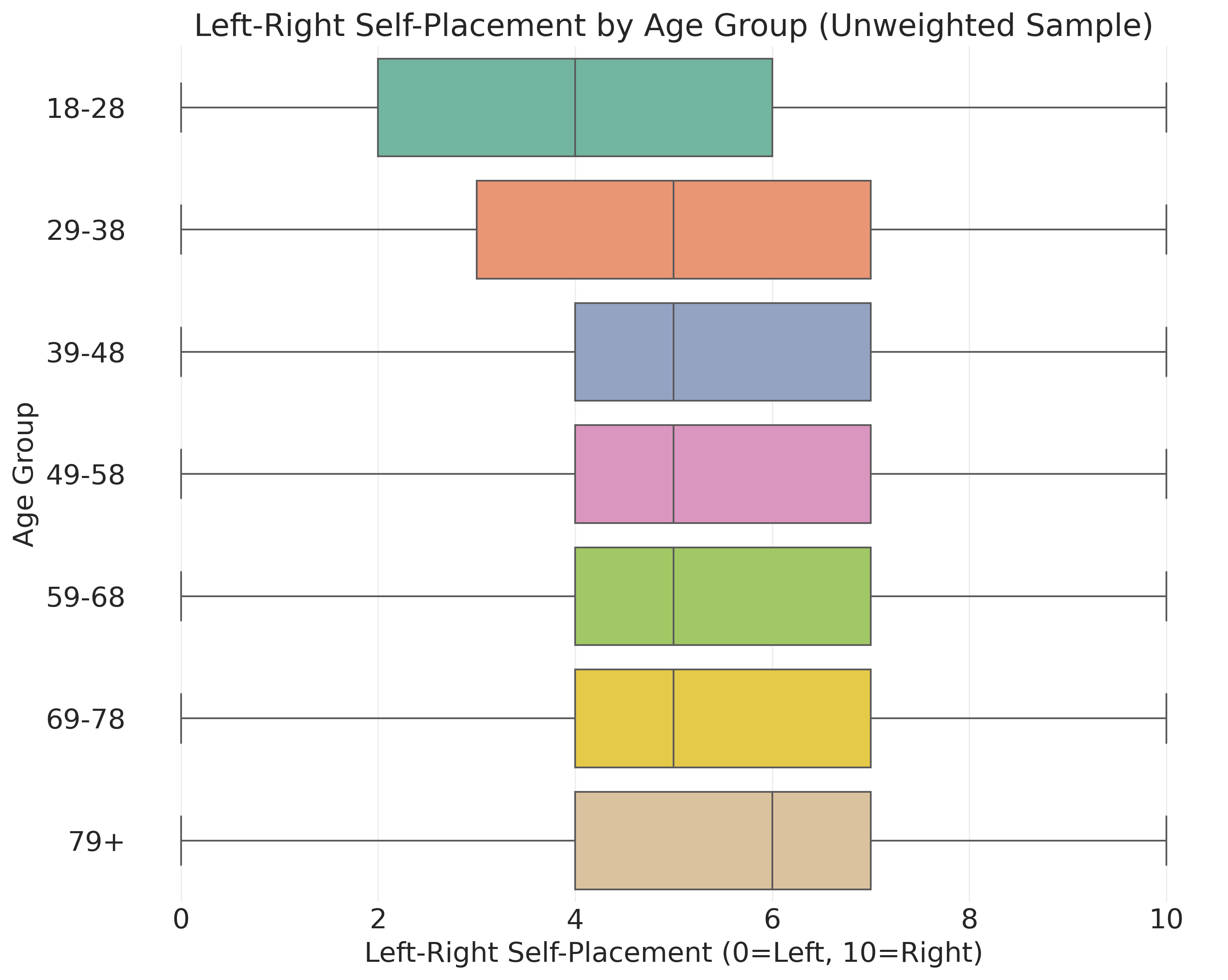
Box plots show five key statistics for each group. The bottom line represents the 25th percentile, where the bottom quarter of responses fall. The box itself extends from the 25th to the 75th percentile, containing the middle half of responses. The dark line inside the box marks the median or 50th percentile. The top line represents the 75th percentile, where the top quarter of responses fall. Dots beyond the lines indicate outliers or unusually extreme values.
When reading the pattern, if the median line moves up as age increases, it suggests older people tend toward higher values or more conservative positions. The box height shows variability. Tall boxes mean lots of disagreement within that age group, while short boxes indicate more consensus.
6.4.4 Continuous by Categorical: Political Ideology by Education Level
Let’s explore how left-right political placement varies across education levels using box plots:
# Prepare data grouped by education level
lr_by_education = []
education_level_labels = []

for edu_code in sorted(ces_clean["cps21_education"].dropna().unique()):
    # Filter to valid left-right responses (0-10 scale) for this education level
    lr_scores = ces_clean[
        (ces_clean["cps21_education"] == edu_code)
        & (ces_clean["cps21_lr_scale_bef_1"] >= 0)
        & (ces_clean["cps21_lr_scale_bef_1"] <= 10)
    ]["cps21_lr_scale_bef_1"].dropna()

    if len(lr_scores) > 0:  # Only include levels with at least one observation
        lr_by_education.append(lr_scores.values)
        education_level_labels.append(
            education_labels.get(int(edu_code), f"Code {int(edu_code)}")
        )

# Create horizontal boxplot
fig, ax = plt.subplots(figsize=(12, 8))
bp = ax.boxplot(lr_by_education, vert=False, patch_artist=True)

# Style the plot
for median in bp["medians"]:
    median.set(color="black", linewidth=2)

colors = plt.cm.RdBu_r(np.linspace(0, 1, len(lr_by_education)))
for patch, color in zip(bp["boxes"], colors):
    patch.set_facecolor(color)
    patch.set_alpha(0.7)

ax.set_yticklabels(education_level_labels)
ax.set_xlabel("Left-Right Placement (0=Left, 10=Right)")
ax.set_title("Political Ideology by Education Level\n(Unweighted Sample)")
ax.axvline(5, color="gray", linestyle="--", alpha=0.5, linewidth=1)  # Mark center
plt.tight_layout()
plt.show()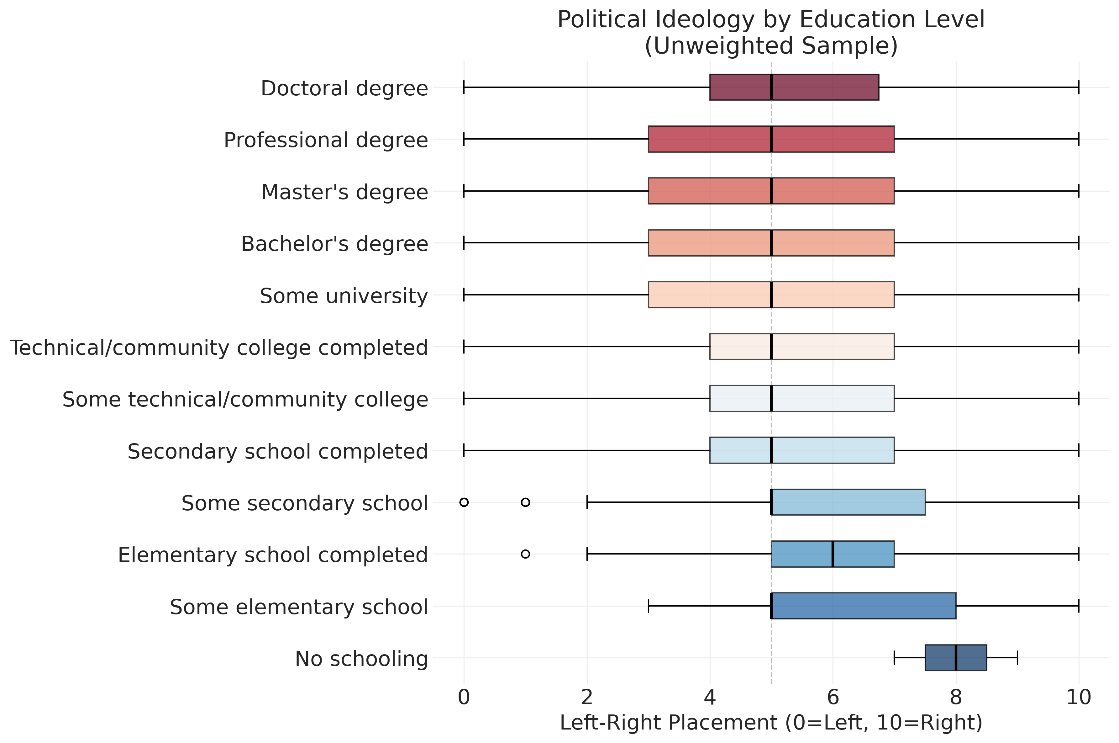
6.5 Choosing the Right Visualization
Understanding basic measurement scales (?sec-measurement-scales) is foundational for data visualization. Categorical variables (nominal and ordinal) and continuous variables (interval and ratio) have different requirements. Matching visualization to measurement type is part of communicating about the patterns in your data clearly and honestly.
Different types of data require different visualization approaches. Bar charts work best for categorical data, showing frequencies or percentages for things you can count like party preference, education level, or province. They make it easy to compare categories at a glance. Histograms work best for continuous data, showing the shape of your data distribution for things you can measure like age, income, or survey completion time. They reveal patterns like skewness or multiple peaks that indicate distinct subgroups.
Box plots are particularly useful for comparing continuous variables across groups. They show the median as a middle line, quartiles as box edges, and outliers as dots. They’re perfect for answering questions like “Does income vary by education level?” and provide a compact way to compare distributions across multiple categories. Scatter plots work best for relationships between two continuous variables, with each point representing one person’s values on both variables. They show correlation patterns visually and make it easy to spot trends, clusters, or outliers.
When dealing with large datasets, hexbin plots often work better than scatter plots. They show density of observations rather than individual points, revealing patterns hidden by overlapping data. Instead of seeing thousands of stacked dots, you see which combinations are most common and which are rare.
The key is matching your chart type to your question. When comparing categories, use a bar chart. When exploring a distribution, use a histogram. When comparing groups, use a box plot. When exploring relationships, use a scatter plot. When dealing with overplotting, use a hexbin plot.
6.6 Interpreting Basic Relationships
When we observe relationships in survey data, we must be careful about interpretation. Correlation does not imply causation. Just because two variables are related doesn’t mean one causes the other. There may be third variables that explain both, or the relationship may be coincidental.
This is one of the most important principles in data analysis. Consider the age and ideology relationship we observed. If older people are more conservative, this could mean several different things. It might reflect a life cycle effect where people become conservative as they age, with aging causing conservatism. It might reflect a generational effect where today’s older people grew up in different times, reflecting their cohort rather than aging per se. It might reflect a selection effect where more liberal older people don’t participate in surveys, creating sampling bias. It might reflect a period effect where recent events affected age groups differently, capturing a specific historical moment rather than a general pattern.
Consider another example. Imagine we find that people who drink more coffee score higher on political knowledge tests. This correlation could reflect several mechanisms. It might be a direct effect where caffeine improves cognitive performance on the test. It might reflect a third variable where highly educated people both drink more coffee and know more about politics for independent reasons. It might reflect reverse causation where people interested in politics stay up late reading news and drink coffee to stay alert. It might be a spurious correlation where coffee drinking and political knowledge both correlate with age, income, or urban residence, creating an apparent relationship with no direct connection.
We should use multiple types of evidence, control for alternative explanations, and be humble about causal claims. Correlation is the starting point for investigation, not the ending point. Good research treats observed relationships as puzzles to be explained rather than conclusions to be announced.
The visualizations we created reveal a relationship between age and political ideology among survey participants. The correlation of 0.125 is weak, meaning age explains only about 1.6% of the variance in ideology (r² = 0.016). Substantively, older respondents tend to place themselves slightly more to the right, but there’s enormous variation at every age. Practically, knowing someone’s age tells you almost nothing about their ideology. We must also exercise caution because this relationship describes survey participants, not the general population. Age-related response bias could influence this pattern.
For example, if we find that older people place themselves further to the right on the left-right scale, this could reflect life cycle effects where people become more conservative as they age. It could reflect generational effects where current older generations grew up in eras that fostered conservative values. It could reflect period effects where recent political events have differentially affected different age groups. It could reflect selection effects where more liberal older people may be less likely to participate in surveys. Survey data alone cannot distinguish between these explanations without additional information or research designs that can isolate specific mechanisms.
6.7 Understanding Survey Weights: From Sample to Population
So far, we’ve analyzed the unweighted sample, treating each respondent equally. But this creates a problem: not everyone in Canada had an equal chance of being in our sample, and not all types of people responded at the same rates.
The core problem is that your survey sample rarely mirrors the population perfectly. Common distortions include geographic issues where small provinces are often oversampled to ensure sufficient sample sizes for regional analysis. Demographic distortions occur because highly educated people respond to surveys at higher rates than less educated people. Age differences emerge because older people are often easier to reach and more likely to participate. Political interest creates bias because people who care about politics are more likely to complete political surveys.
Survey weights adjust for these distortions by giving more “weight” to underrepresented groups and less weight to overrepresented groups. This allows us to rebalance the sample to better reflect the population we want to study.
Let’s work through a simplified example. Imagine we surveyed 6 people from three age groups, and each person placed themselves on a left-right scale:
# Create a simplified example with 6 respondents
example = pd.DataFrame({
    'Respondent': ['A', 'B', 'C', 'D', 'E', 'F'],
    'Age_Group': ['18-35', '18-35', '36-55', '36-55', '56+', '56+'],
    'Ideology': [3, 4, 5, 6, 7, 8]
})
example| Respondent | Age_Group | Ideology | |
|---|---|---|---|
| 0 | A | 18-35 | 3 |
| 1 | B | 18-35 | 4 |
| 2 | C | 36-55 | 5 |
| 3 | D | 36-55 | 6 |
| 4 | E | 56+ | 7 |
| 5 | F | 56+ | 8 |
Our sample has equal numbers from each age group (33% each), but the actual population has a different age distribution:
# Show the mismatch between sample and population
comparison = pd.DataFrame({
    'Age_Group': ['18-35', '36-55', '56+'],
    'Population_%': [40, 35, 25],
    'Sample_%': [33.3, 33.3, 33.3],
    'Problem': ['UNDER-represented', 'About right', 'OVER-represented']
})
comparison| Age_Group | Population_% | Sample_% | Problem | |
|---|---|---|---|---|
| 0 | 18-35 | 40 | 33.3 | UNDER-represented |
| 1 | 36-55 | 35 | 33.3 | About right |
| 2 | 56+ | 25 | 33.3 | OVER-represented |
The unweighted mean treats everyone equally: (3+4+5+6+7+8) ÷ 6 = 5.50
But since older people (who have higher ideology scores) are overrepresented, this doesn’t reflect the population. Weights correct this by counting underrepresented groups more and overrepresented groups less:
# Calculate weights: population % ÷ sample %
weights_by_group = pd.DataFrame({
    'Age_Group': ['18-35', '36-55', '56+'],
    'Weight': [40/33.3, 35/33.3, 25/33.3],
    'Meaning': ['Count 20% MORE', 'Count 5% MORE', 'Count 25% LESS']
})
weights_by_group.round(2)| Age_Group | Weight | Meaning | |
|---|---|---|---|
| 0 | 18-35 | 1.20 | Count 20% MORE |
| 1 | 36-55 | 1.05 | Count 5% MORE |
| 2 | 56+ | 0.75 | Count 25% LESS |
# Apply weights to calculate population-adjusted mean
example["Weight"] = example["Age_Group"].map(
    {"18-35": 1.20, "36-55": 1.05, "56+": 0.75}
)
weighted_mean = np.average(example["Ideology"], weights=example["Weight"])

weighting_summary = f"""
Weighting Comparison:
  Unweighted mean: 5.50 (treats all 6 people equally)
  Weighted mean:   {weighted_mean:.2f} (adjusts to match population age distribution)

  Difference: {weighted_mean - 5.50:.2f} points
  Interpretation: Younger, more liberal people are under-counted in the unweighted analysis
"""
print(weighting_summary)
Weighting Comparison:
  Unweighted mean: 5.50 (treats all 6 people equally)
  Weighted mean:   5.20 (adjusts to match population age distribution)

  Difference: -0.30 points
  Interpretation: Younger, more liberal people are under-counted in the unweighted analysis
6.7.1 Real Survey Weights Are More Complex
The CES uses sophisticated weighting that adjusts for province and region to ensure each province contributes proportionally to its population, age and sex to match population demographics from Statistics Canada, education level to correct for the fact that educated people respond more often, language to balance English and French respondents appropriately, and household size to account for selection probabilities within households.
The CES provides pre-calculated weights like cps21_weight_general_all that handle all this complexity. When we want to make claims about Canadian voters, we’ll use these weights. When we want to understand how variables relate to each other or test measurement approaches, we often don’t need weights because we’re asking questions about relationships rather than population proportions.
6.7.2 When We’ll Apply Real Weights
In later chapters, particularly when we examine ideological constraint and affective polarization, we’ll learn to apply CES weights properly. For now, the key takeaways are straightforward. Unweighted analysis describes your sample but doesn’t represent the population. Weighted analysis estimates population characteristics but requires understanding survey design. Different research questions require different approaches to weighting. Always be explicit about whether your results are weighted or unweighted, as this fundamentally shapes what claims you can make.
For exploratory analysis focused on understanding variable relationships and measurement quality, like we’ve done here, unweighted analysis is perfectly appropriate and often preferred. The patterns we observe in relationships between variables often hold whether we weight or not, while population proportions can shift substantially.
6.8 Looking Forward: From Exploration to Modeling
This chapter focused on essential skills for exploratory data analysis using data from surveys. You can now conduct univariate and bivariate analyses, create effective visualizations, understand the sample-population distinction, and interpret correlational relationships with appropriate caution. But exploration is just the start. Next, we move from description to formal modeling.
Distinguishing Description from Modeling
The exploratory analyses in this chapter describe patterns in our data: what we observe about age, ideology, education, and their relationships. We calculated correlations, created visualizations, and summarized distributions. These are fundamentally descriptive activities in the sense that they tell us what our sample looks like; they don’t formalize relationships, make predictions, or quantify uncertainty.
In the next three chapters, we transition to analytical modeling:
Regression models (?sec-regression) formalize relationships between predictors and outcomes, allowing us to control for multiple variables simultaneously, make predictions with quantified uncertainty, and test theoretical hypotheses about which variables matter most.
Logistic regression models (?sec-logistic-regression) extend these ideas to binary outcomes (voted/didn’t vote, supports policy/opposes it), using specialized models that respect the categorical nature of the outcome while maintaining interpretability.
Count models (?sec-glms-counts) handle situations where our outcome is a count (number of protests attended, number of news sources consulted), requiring models that respect the non-negative, integer nature of count data.
Why Models Formalize What Exploration Reveals
Exploratory analysis reveals patterns worth investigating—we found that age and ideology correlate weakly, that education varies by region, and that political attitudes show substantial individual variation. But these observations raise questions that exploration alone cannot answer:
- How much does each predictor contribute when we consider multiple variables together? (Age might correlate with ideology, but what happens when we control for education, income, and region?)
- How confident should we be in our estimates? (The correlation of r = 0.122 came from our sample—how much uncertainty is there around that value if we want to make claims about the population?)
- What predictions can we make? (If we know someone’s age, education, and region, what’s our best guess about their political ideology, and how uncertain is that guess?)
Models provide a formal framework for answering these questions. They quantify uncertainty through credible intervals, control for confounding by including multiple predictors, and make explicit the assumptions underlying our inferences.
Motivating Uncertainty Quantification and Prediction
Throughout the upcoming chapters, we’ll maintain a Bayesian perspective that treats parameters as uncertain quantities to be described with probability distributions. This is a natural extension of our exploratory mindset: just as we described the distribution of age or ideology in our sample, we’ll describe the distribution of plausible parameter values (slopes, intercepts, effect sizes) given our data.
Bayesian models provide:
- Credible intervals that directly quantify our uncertainty about parameters
- Posterior distributions that show the full range of plausible parameter values
- Predictive distributions that incorporate both sampling variability and parameter uncertainty
- Intuitive interpretations that avoid the logical contortions of null hypothesis significance testing
We’ll use the same data, the same variables, and the same substantive questions—but now with tools that let us move from “these variables are related” to “this is how strongly they’re related, with this much uncertainty, controlling for these other factors.”
The solid foundation we’ve built, from data collection and processing through exploratory analysis, now enables the sophisticated theoretical work that makes quantitative social science both scientifically rigorous and substantively meaningful. In ?sec-regression, we’ll start by formalizing the age-ideology relationship we explored here into a regression framework that quantifies uncertainty and supports causal reasoning.