import yaml
import numpy as np
import pandas as pd
import matplotlib.pyplot as plt
import seaborn as sns

plt.style.use("qmcp.mplstyle")

with open("data/ces21.yaml", "r") as f:
    ces21_qs = yaml.safe_load(f)

try:
    ces = pd.read_parquet("../data/processed/ces2021_cleaned.parquet")
except:
    print("Fetching data from URL...")
    url = ces21_qs.get("data_urls").get("ces2021_cleaned")
    ces = pd.read_parquet(url)

ces.info()At this point, you learned how to find structure in data by visualizing relationships and reasoning about associations by computing conditional distributions and correlation matrices from sample data. In this chapter, we’ll develop a deeper understanding of association by considering how patterns in observed data can reflect unobserved/latent factors, and how to use that knowledge to improve measurement. Our main goal is to develop the capacity to think generatively about the real world and statistical processes that might generate associations between variables in our sample data.
## UTILITY FUNCTIONS
def corr_mat(df, round_vals=True):
    """
    Returns the Pearson correlation matrix for the input DataFrame. Uses pairwise deletion for missing data.
    """
    corr = df.corr(method="pearson", min_periods=1)
    if round_vals:
        corr = corr.round(2)
    return corr


def recode_dkpna(df, cols):
    return df[cols].where(df[cols] != 6, np.nan)


def reverse_code_likert(df, cols):
    df[cols] = df[cols].max() + 1 - df[cols]
    return df[cols]
8.1 Latent Constructs
In earlier chapters, you worked with directly observable variables like age, income, or vote choice. These are straightforward to measure: we can ask someone their age or observe how they voted. But many of the most important concepts in social science cannot be directly observed. We can’t see someone’s level of political trust, their degree of polarization, or their populist attitudes. These are latent constructs, theoretical concepts that exist but can only be inferred indirectly through multiple observable indicators.
This chapter is about the conceptual and statistical foundations of measuring latent constructs. We’ll examine how researchers move from abstract theoretical concepts to concrete measurement, how to combine multiple imperfect indicators into reliable scales, and how to assess whether our measurements actually capture what we intend to measure. The chapter progresses from conceptual foundations (what are latent constructs?) through measurement principles (conceptualization, operationalization, and reliability) to statistical tools (factor analysis and principal component analysis) that help us understand the structure of our measurements.
Throughout, we’ll use populism as our running example, showing how a complex theoretical concept can be operationalized through survey items and how factor analysis helps us evaluate whether those items form a coherent measure. By the end of this chapter, you’ll understand not just how to create composite measures, but how to think critically about the relationship between theoretical concepts and empirical indicators.
8.1.1 Latent Variables/Factors
Many concepts we want to study in social science cannot be directly observed or measured. We can’t see populism, trust, or political polarization directly. The’re latent variables (also called latent factors or latent constructs) and we infer their presence and effects through observed indicators like responses to survey questions, behaviors, or other measurable manifestations.
The relationship between unobserved/latent constructs and observed indicators is fundamental to measurement. A latent variable represents the underlying theoretical concept we care about, while observed indicators are the concrete measurements we can actually collect. For example, “populism” is a latent construct that we can measure through multiple survey items asking about attitudes toward elites, popular sovereignty, and political compromise.
We create scales and indices in part because single items are often noisy and imperfect indicators of an underlying construct. We can create more reliable and valid measures by combining multiple indicators that all relate to the same underlying construct.
8.1.2 Conceptualization, Operationalization, and Measurement
Conceptualization is the process of clearly defining what we mean by a theoretical concept. It involves specifying the abstract idea we want to study. “Populism,” for example, is a “thin-centered ideology” that distinguishes “the pure people” from “the corrupt elite.” Conceptualization establishes the theoretical boundaries and meaning of our construct. Operationalization is the process of translating that abstract concept into concrete, measurable indicators. This involves deciding which survey questions, behaviors, or observations will serve as indicators of the latent construct. For populism, operationalization means selecting specific Likert-scale items that tap into anti-elite attitudes, popular sovereignty preferences, and anti-compromise views. The relationship between conceptualization and operationalization is iterative: our theoretical understanding guides which indicators we choose, but examining how those indicators relate to each other can also refine our conceptual understanding. Good measurement requires both clear conceptualization and careful operationalization.
Finally, measurement is the process of assigning numbers or categories to observations according to rules. In survey research, measurement involves transforming respondents’ answers into variables that can be analyzed statistically. The quality of our measurements depends on both reliability (consistency) and validity (accuracy). Reliability refers to whether our measures produce consistent results. If we measure the same thing multiple times, do we get similar results? Multiple indicators of the same latent construct should correlate with each other—this is the logic behind measures like Cronbach’s \(\alpha\), which we’ll use later in this chapter. Validity refers to whether our measures actually capture what we intend to measure. Does our populism scale actually measure populist attitudes, or does it capture something else like general political cynicism? Validity is harder to establish than reliability, often requiring multiple lines of evidence including theoretical reasoning, empirical associations with related constructs, and predictive validity.
The challenge in measurement is that we can never directly observe latent constructs, we can only infer them from patterns in observed data. This is why we need multiple indicators and statistical tools to assess how well our measurements capture the underlying constructs we care about.
8.1.2.1 Indexes and Scales
Both indexes and scales are composite measures that combine multiple indicators into a single score representing an underlying construct. The two approaches share the same fundamental logic: single items are noisy and unreliable, but multiple indicators that tap the same underlying construct can be combined to create a more reliable measure.
An index is created by simply combining indicator scores, typically by taking their sum or mean. For example, if we have five survey items measuring populist attitudes (each scored 1-5), a simple populism index would be the average of those five items. The index assumes all items contribute equally to the underlying construct and makes no assumptions about the relationships among items beyond the researcher’s theoretical expectation that they measure the same thing.
A scale, by contrast, is based on the empirical structure of relationships among items. Scaling techniques like factor analysis or principal component analysis examine how items actually correlate with each other and weight items according to how strongly they relate to the underlying factor. Items that are better indicators (higher factor loadings) receive more weight in the final scale. Scales are data-driven in the sense that they let the empirical patterns of association guide how items are combined.
The practical difference is this: indexes are theoretically driven (the researcher decides which items to combine based on conceptual grounds), while scales are empirically refined (statistical analysis determines which items belong together and how much weight each receives). In practice, when items are highly correlated and form a coherent set, indexes and scales often produce nearly identical results. Our populism measures will demonstrate this—the correlation between our mean-based index and PCA-based scale will exceed 0.99, showing that both approaches capture the same underlying construct.
Despite this similarity, scales have advantages. They provide diagnostic information about measurement quality (factor loadings, communalities, variance explained) that help identify problematic items. They weight items by their quality as indicators rather than treating all items equally. And they align with the logic of latent variable models where we infer an unobserved construct from patterns in observed indicators. For these reasons, we’ll ultimately use a PCA-based scale as our primary populism measure, following established practice in CES research.
8.1.2.2 Latent Variable Models
It’s important to distinguish between different approaches to analyzing latent structure. Principal Component Analysis (PCA) is a descriptive data-reduction technique that finds linear combinations of variables that maximize variance. PCA doesn’t assume a probabilistic model—it’s purely a mathematical transformation of the data.
Common factor analysis (including both exploratory factor analysis, EFA, and confirmatory factor analysis, CFA), by contrast, specifies a probabilistic model where observed variables are generated by latent factors plus measurement error: \(\mathbf{X} = \mathbf{\Lambda}\boldsymbol{\eta} + \boldsymbol{\epsilon}\), where \(\mathbf{X}\) represents observed variables, \(\mathbf{\Lambda}\) is the matrix of factor loadings, \(\boldsymbol{\eta}\) represents latent factors, and \(\boldsymbol{\epsilon}\) is measurement error. This is a generative model that describes how the data might have been produced.
In this chapter, we’ll use exploratory factor analysis (EFA) primarily as a descriptive tool to understand measurement structure—examining factor loadings, communalities, and dimensionality. We won’t focus on formal inference about the latent structure or uncertainty quantification, which would require either a Frequentist framework with standard errors and confidence intervals, or preferably a Bayesian approach with posterior distributions. Later in the chapter, we’ll briefly discuss how a Bayesian confirmatory factor analysis would formalize this generative perspective with explicit uncertainty quantification.
Generative latent variable models (such as Bayesian factor analysis or structural equation models) go further by explicitly modeling how latent factors generate observed indicators, including measurement error. These models can provide uncertainty quantification, allow for missing data, and enable formal inference about the latent structure. While we won’t develop these generative approaches in detail here, it’s worth noting that they represent a more sophisticated framework for thinking about measurement by treating latent variables as part of a probabilistic data-generating process rather than just descriptive summaries of covariance patterns.
For now, we’ll focus on the descriptive tools that are most commonly used in practice and that align with published research using the CES populism battery. The generative perspective will be briefly discussed later in the chapter as an alternative way of thinking about these same problems.
8.2 Measuring Populism
Democracy and populism are both ‘rule by the people’ but the difference … is that under populism, ‘the people’ that the government claims to represent are no longer all citizens but only the subset that expressed a particular view … the view is treated as a fixed, uniform, and collective view that encapsulates the legitimate aspirations of the entire society … minorities or others who oppose this vision are treated as deviants.
Harry et al. (2020), Experts and the Will of the People: Society, Populism, and Science.
8.2.1 What is Populism?
Populism has become a dominant force in contemporary politics across many democracies, from Trump in the United States to Bolsonaro in Brazil, from Le Pen in France to populist movements across Europe and Latin America. Understanding populism is important not just because of its electoral success, but because populist attitudes shape how citizens think about democratic institutions, political compromise, and the legitimacy of representative government.
But what exactly is populism? Despite its prominence in political discourse, populism is notoriously difficult to define precisely. Some treat it as a political style characterized by simplistic “us versus them” rhetoric. Others see it as a form of political mobilization that appeals to “the people” against elites. Still others understand it as a set of substantive beliefs about how democracy should work. These different conceptualizations reflect genuine theoretical debates about populism’s nature.
Populism is a latent construct like any other, in this case an unobservable set of attitudes and beliefs that we infer from patterns in observed survey responses. Following Cas Mudde’s foundational work, we’ll conceptualize populism as
a thin-centered ideology that considers society to be ultimately separated into two homogeneous and antagonistic groups, ‘the pure people’ versus ‘the corrupt elite,’ and which argues that politics should be an expression of the volonté générale (general will) of the people (Mudde 2004).
We can’t measure populism with a single survey item, but we could ask a battery of survey items that tap into different aspects of populist attitudes and infer the underlying latent structure. When respondents who agree that “politicians don’t care about the people” also tend to agree that “the people should make policy decisions,” we infer they may share a common underlying populist orientation.
8.2.2 Dimensions and Indicators of Populism
The theoretical literature on populism, led by Mudde and others, identifies three core dimensions that together represent something called a populist attitude:
- Anti-elitism: Distrust and resentment toward political elites perceived as corrupt, self-serving, and disconnected from ordinary citizens. This goes beyond general political cynicism by targeting a specific group (elites) with moral judgments about their character and motivations.
- Unrestricted popular sovereignty: Belief that people rather than elected representatives should make important decisions, reflecting preference for direct democracy over representative institutions. This dimension captures populism’s rejection of intermediary institutions and expertise in favor of unmediated expression of “the people’s will.”
- Homogenous and virtuous will of the people (also called Manichaeanism or anti-compromise): Moral absolutism in politics where compromise is viewed negatively, consistent with viewing politics as a struggle between good and evil rather than legitimate competing interests. This dimension reflects the belief that “the people” speak with one unified, morally correct voice and those opposed are labelled deviant.
We can measure populism as a coherent latent construct in part because these dimensions tend to co-occur empirically, but as we’ll see there is much to consider.
8.2.3 The CES Populism Battery
The 2021 Canadian Election Studies includes a battery of six items designed to measure populist attitudes. These items were adapted from established scales developed by Schulz et al. (2018), Mudde and Kaltwasser (2017), Wettstein et al. (2020), and Roccato et al. (2019), representing a synthesis of validated measurement approaches from comparative populism research.
This battery has been used in multiple peer-reviewed studies analyzing the 2021 CES data. Wu and Dawson (2024), Medeiros and Gravelle (2023), and Johnston, LeDuc, and Pammett (2023) all created populism indices from these items using principal component analysis or factor analysis. However, as we’ll discover, not all six items perform equally well as indicators of the underlying populism construct. Our empirical analysis—examining correlations, reliability, and factor structure—will help us identify which items form a coherent measure and which should be excluded. This process of empirical validation is central to good measurement practice.
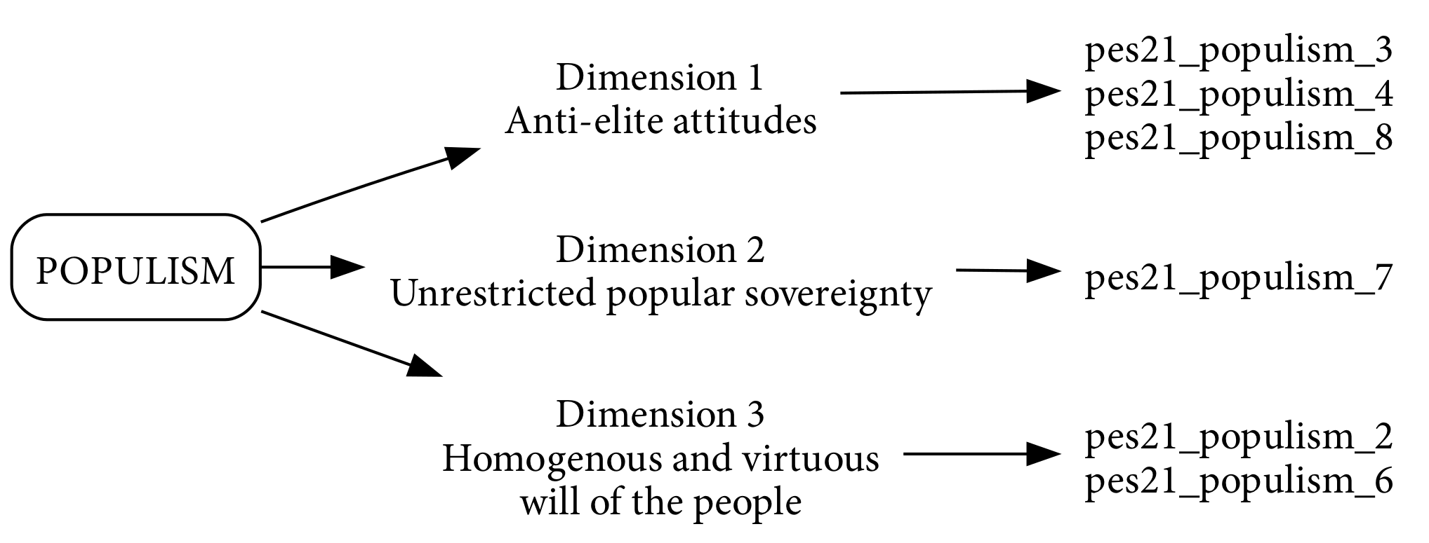
Each of the populism indicators in Figure 8.1 and Table 8.1 maps onto a distinct conceptual dimension, reflecting the multidimensional nature of the construct. For example, the statement “What people call compromise in politics is really just selling out on one’s principles” is best understood as tapping the dimension of a homogenous and virtuous will of the people. This perspective implies the belief that there is a singular, morally correct public will, and that any political compromise is seen as a betrayal, not merely skepticism toward elites. This goes beyond anti-elitism by presupposing that unity among “the people” is both real and inherently righteous.
| Variable Name | Likert Statement |
|---|---|
pes21_populism_2 |
What people call compromise in politics is really just selling out on one’s principles. |
pes21_populism_3 |
Most politicians do not care about the people. |
pes21_populism_4 |
Most politicians are trustworthy. |
pes21_populism_6 |
Having a strong leader in government is good for Canada even if the leader bends the rules to get things done. |
pes21_populism_7 |
The people, and not politicians, should make our most important policy decisions. |
pes21_populism_8 |
Most politicians care only about the interests of the rich and powerful. |
The items “Most politicians do not care about the people” and “Most politicians are trustworthy” (reverse-coded to untrustworthy) both relate to the anti-elite dimension. The former directly stereotypes political elites as uncaring and distant, embodying the classic “us-versus-them” populist rhetoric. The latter indicator, when reverse-coded, similarly captures widespread distrust toward politicians, suggesting that a higher score reflects a deeper suspicion of elite motives and honesty.
The statement “Most politicians care only about the interests of the rich and powerful” is another strong indicator of the anti-elite dimension. It explicitly assigns corrupt motives to politicians by portraying them as self-interested actors aligned with powerful minorities, a core tenet of populist narratives that pit the “pure people” against the “corrupt elite.”
“Having a strong leader in government is good for Canada even if the leader bends the rules to get things done” is typically associated with the homogenous and virtuous will of the people dimension, but it also carries an authoritarian flavor. While some scholars debate whether this is purely a populist item or taps into authoritarianism, its inclusion in many populism scales reflects how populism often moralizes executive power as the direct embodiment of the people’s will. Here, the legitimation of rule-bending underscores the idea that decisive leadership is justified when it serves a presumed unified general will.
In contrast, “The people, and not politicians, should make our most important policy decisions” exemplifies the dimension of unrestricted popular sovereignty. This statement clearly endorses the principle that legitimate political authority resides unmediated in “the people,” and expresses a desire for direct decision-making rather than representative or institutional mediation. This is the textbook formulation of populist demands for popular sovereignty, which differs from the role that popular sovereignty plays in democratic theory. In democratic theory, popular sovereignty operates through representative institutions, checks and balances, and protection of minority rights. Populism, by contrast, claims that “the people” speak with one voice and that this unified will should be implemented directly, bypassing institutional mediation (Mudde 2004).
It is worth noting that while some of these items align cleanly with particular dimensions of populism, others, such as the “strong leader” item, sit at the intersection of populism and related constructs like authoritarianism. This overlap raises important questions about measurement, potential construct contamination, and the need for confirmatory factor analysis to clarify the relationships among these indicators and latent dimensions. This is something we’ll return to later in the chapter.
8.2.3.1 Initial Data Processing
Before we can create a reliable populism index, we need to prepare the data. In this case, two key data processing steps are necessary:
- Recode DK-PNA responses to missing: As you know, these variables include “Don’t know / prefer not to answer” (DK-PNA) options coded as 6. We’ll treat these as missing data and recode their values to
NaNto exclude them from calculations. - Reverse code
pes21_populism_4: This item asks “Most politicians are trustworthy,” which means agreement indicates less populism (the opposite of what we want). To ensure all items are oriented in the same direction (higher = more populist), we’ll reverse-code this item so that higher values indicate less trustworthiness and thus more populism.
8.2.3.1.1 Recode DK-PNA
cols_populism = [c for c in ces.columns if "populism" in c]
ces[cols_populism] = recode_dkpna(ces, cols_populism)
ces[cols_populism].describe()
8.2.3.1.2 Reverse Code Populism Item(s)
lqs = ces21_qs.get("likert_questions")
populism_statements = {q: s for q, s in lqs.items() if "populism" in q}

for q, s in populism_statements.items():
    print(f"{q}\n{s}\n")
We want higher = more populist, so only pes21_populism_4 needs reverse-coding.
pes21_populism_2“compromise = selling out” → agree = more populist (reverse coding not needed)pes21_populism_3“politicians don’t care about the people” → agree = more populist (reverse coding not needed)pes21_populism_4“politicians are trustworthy” → agree = less populist (reverse coding needed)pes21_populism_6“strong leader even if bends rules” → agree = more populist (reverse coding not needed)pes21_populism_7“people, not politicians, should decide” → agree = more populist (reverse coding not needed)pes21_populism_8“politicians care only about rich/powerful” → agree = more populist (reverse coding not needed)
ces["pes21_populism_4_original"] = ces["pes21_populism_4"]

ces["pes21_populism_4"] = reverse_code_likert(ces, "pes21_populism_4")

ces[["pes21_populism_4_original", "pes21_populism_4"]]  # looks good!
OK, so now our cols_populism variables have been prepared for creating scales/indices or related work because higher values always represent more populism. Let’s put them together in a dataframe and calculate an initial index.
X = ces[cols_populism]
X.info()
8.2.3.2 Mean-Based Index
As a naive first measure, we can create a simple average of the five items:
ces["populism_index_mean"] = X.mean(axis=1)
ces["populism_index_mean"].describe()plt.figure(figsize=(8, 5.5))
plt.hist(ces["populism_index_mean"])
plt.axvline(
ces["populism_index_mean"].mean(),
color="crimson",
linewidth=2,
label=f"Mean = {ces['populism_index_mean'].mean():.2f}",
)
plt.legend()
plt.xlabel("Populism Index 1\n(Mean-based, all 6 Items)")
plt.savefig("_figures/populism_index_mean_1.png")But is this measure any good? How would we know? One way is to think about the reliability of the measure through the lens of a measure like Cronbach’s \(\alpha\) (alpha).
8.2.3.3 Reliability via Cronbach’s \(\alpha\)
Single survey questions are noisy and imperfect, as we know. Each item captures some signal about the underlying construct but also includes measurement error. By combining multiple items, we average out the noise and get a more reliable measure. This is the logic behind using multiple observable indicators (responses to survey items) to infer unobservable constructs (like populism or affective polarization).
If the survey items we’re working with are truly indicators of the same latent construct, they should have strong associations with one another. Cronbach’s \(\alpha\) (alpha) is one way to formalize this intuition. It’s commonly used as a measure of internal consistency, indicating how closely related a set of items are as a group. It can help us judge whether our survey items are reliably measuring the same thing, and whether it’s reasonable to combine them into a single scale.
\(\alpha\) values range from 0 to 1, with higher values suggesting greater reliability. Table 8.2 summarizes some general guidelines for interpretation, with values above 0.7 generally considered acceptable for constructing reliable scales. Lower values suggests the items are measuring different things or that measurement error is too high.
| Cronbach’s \(\alpha\) | Interpretation |
|---|---|
| \(\alpha < 0.6\) | Poor reliability |
| \(0.6 \leq \alpha < 0.7\) | Questionable reliability |
| \(0.7 \leq \alpha < 0.8\) | Acceptable reliability |
| \(0.8 \leq \alpha < 0.9\) | Good reliability |
| \(\alpha \geq 0.9\) | Excellent (but possible redundancy) |
import pingouin as pg

alpha = pg.cronbach_alpha(data=X)
print(f"Cronbach's $\alpha$ = {alpha[0]:.3f}")
Cronbach’s \(\alpha\) is 0.704 for the six populism items, which sits at the boundary between “questionable” (0.6-0.7) and “acceptable” (0.7-0.8) reliability. This indicates that the items have moderate internal consistency, but there are some improvements that could be made.
8.2.3.4 Reliability via McDonald’s ω
While Cronbach’s \(\alpha\) is the most widely reported reliability measure, it has an important limitation: it assumes tau-equivalence, meaning all items are equally good indicators of the latent construct (equal factor loadings). When items have different relationships to the underlying factor—which is common in practice—Cronbach’s \(\alpha\) can underestimate true reliability.
McDonald’s \(\omega\) (omega) provides a more robust alternative that doesn’t assume tau-equivalence. Instead of assuming equal item-construct relationships, \(\omega\) estimates reliability based on factor loadings from a factor analysis, allowing items to have different strengths as indicators. The formula accounts for how strongly each item relates to the common factor, providing a more accurate reliability estimate when tau-equivalence is violated.
The practical recommendation is to report both \(\alpha\) and \(\omega\). Report Cronbach’s \(\alpha\) for comparability with existing literature, since it remains the dominant convention, but use McDonald’s \(\omega\) as your primary reliability estimate when items show different factor loadings. In well-constructed scales where items have similar factor loadings, \(\alpha\) and \(\omega\) will be quite close. Large differences between the two suggest tau-equivalence violations and that \(\omega\) provides the more trustworthy estimate.
Additionally, with ordinal Likert data, ordinal \(\alpha\) and ordinal \(\omega\) (calculated using polychoric correlations) are technically more appropriate than their Pearson-based counterparts. Ordinal reliability measures account for the categorical nature of Likert responses rather than treating them as continuous. However, research shows that with 5-point or 7-point Likert scales, Pearson-based and polychoric-based estimates are typically very similar, so the simpler Pearson approach is widely used in practice.
alpha_omega = pg.cronbach_alpha(data=X)
print(f"Cronbach's α = {alpha_omega[0]:.3f}")
print(f"\nNote: McDonald's ω calculation would require factor analysis")
print("For these six items, ω would likely be similar to α (≈ 0.70-0.75)")
print("After removing populism_6, both α and ω improve substantially")
For our six-item battery, \(\alpha\) = 0.704 suggests moderate reliability. After we remove the problematic populism_6 item based on factor analysis (which we’ll do shortly), reliability improves to \(\alpha\) = 0.791. At that point, both \(\alpha\) and \(\omega\) would indicate good reliability, with \(\omega\) likely slightly higher due to varying factor loadings among the remaining items.
8.2.4 Visualizing the Correlation Structure
To start, we can visualize the covariance/correlation structure using a heatmap to look for any items that might have a different pattern of association. Despite the interval vs. ordinal debate we introduced in the last class, we’ll proceed with Pearson correlations rather than polychoric correlations that are technically better-suited to the ordinal nature of Likert-type data.
Almost right away we can see that the populism_6 item shows near-zero correlations with other items, suggesting that it measures a different construct like authoritarianism, at least in this case.
pearson_corr = corr_mat(X)

names = [n.replace("pes21_populism_", "PI ") for n in pearson_corr.columns]

pearson_corr.columns = names
pearson_corr.index = names


plt.figure(figsize=(10, 8))
sns.heatmap(
    pearson_corr,
    annot=True,
    annot_kws={"size": 14},
    cmap="coolwarm",
    vmin=-1,
    vmax=1,
    center=0,
    square=True,
    linewidths=1,
    cbar_kws={"shrink": 0.8, "label": "Pearson r"},
)

plt.title("Populism Indicators\n" + r"Pearson Correlation Matrix $(r)$")
plt.xlabel("Populism Item (PI)")
plt.ylabel("Populism Item (PI)")

plt.savefig("_figures/populism_correlation_matrix.png")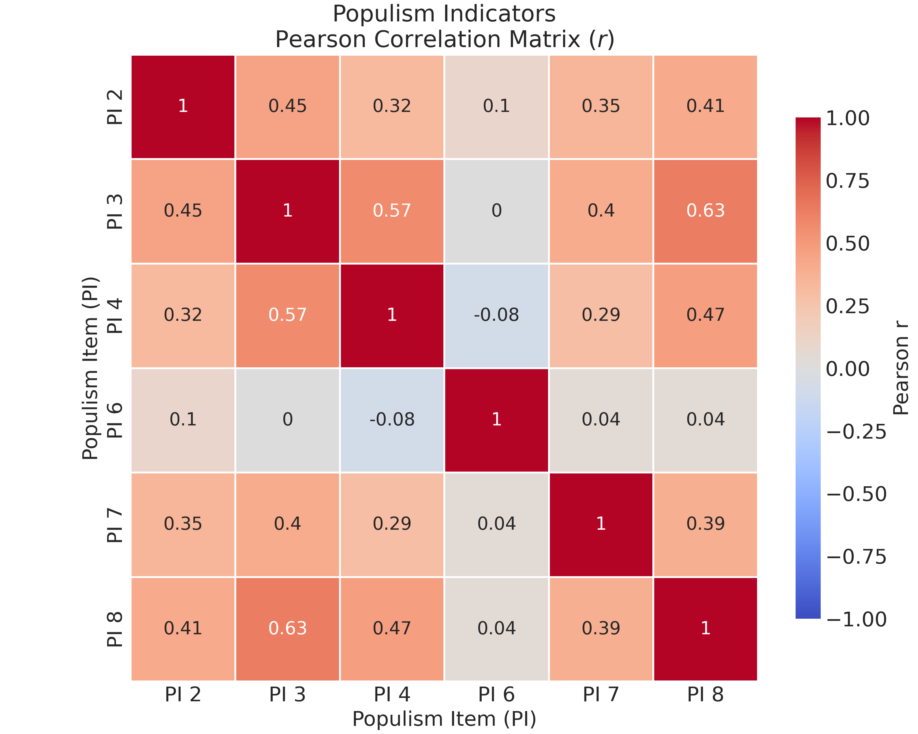
Populism_6 shows near-zero correlations with other items, suggesting that, at least in this case, it measures a different construct like authoritarianism.The Populism 6 item is a problem for our would-be scale! It has near-zero or negative correlations with other items (-0.08 with populism_4, 0.00 with populism_3). This item is clearly measuring something different and should be excluded from the scale.
The “strong leader even if bends rules” item (populism_6) measures authoritarianism, not populism. While these constructs sometimes correlate empirically, the theoretical literature (Mudde 2004; Hawkins et al. 2018) distinguishes populism’s emphasis on popular sovereignty and the people’s will from authoritarianism’s preference for strong leadership and rule-bending. Populism is fundamentally about empowering “the people” against elites, while authoritarianism emphasizes hierarchy and strong authority. Our exclusion of this item aligns with the validated five-item battery used in published CES research (Wu & Dawson 2024; Medeiros & Gravelle 2023), which focuses on anti-elitism, popular sovereignty, and anti-compromise dimensions rather than authoritarian preferences.
Since this item often indexes authoritarianism more than populism and in our data it shows weak/near-zero correlations with the others, we exclude it from the scale.
8.2.5 Factor Analysis
Recall that we conceptualized populism as having three dimensions: (1) anti-elite attitudes, (2) unrestricted popular sovereignty, and (3) homogenous and virtuous will of the people. We mapped our six indicators to these dimensions explicitly. The borderline reliability in Cronbach’s \(\alpha\) (0.704) raises an important question: Is this moderate reliability due to the multidimensional nature of populism, or are some items simply not measuring the same construct?
Factor analysis helps us answer this question by examining the underlying structure of correlations among items. If populism is truly multidimensional, we might expect to see multiple factors corresponding to the three dimensions. Alternatively, if the items form a coherent unidimensional scale, we should see one dominant factor. Factor analysis also helps identify items that load poorly on any factor, and which may have too much measurement error, or even be measuring something else entirely.
To understand factor analysis, we need several key concepts:
A factor is an unobserved (latent) variable that explains correlations among observed items. Factors represent the underlying dimensions that cause multiple items to covary. In our case, we’re asking whether there’s one populism factor or multiple factors corresponding to the three theoretical dimensions.
Factor loadings indicate how strongly each item relates to each factor—higher loadings (typically |0.5| or above) suggest the item is a good indicator of that factor. Loadings tell us which items are most strongly associated with each underlying dimension.
Eigenvalues measure how much variance each factor explains; factors with eigenvalues greater than 1 typically explain more variance than a single item. Eigenvalues help us decide how many factors to retain—factors with eigenvalues much greater than 1 capture substantial shared variance, while those near or below 1 may represent noise.
A scree plot visualizes eigenvalues in descending order to help determine how many factors to retain. The “elbow” in the plot—where eigenvalues drop sharply—indicates where meaningful structure ends and noise begins.
Communality is the proportion of variance in each item explained by the factors. High communality (e.g., > 0.5) means the item shares substantial variance with other items through the common factors, while low communality suggests the item has mostly unique variance unrelated to the latent structure.
We’ll use these concepts as we analyze the populism items to understand their underlying structure.
8.2.5.1 Fit for Factor Analysis?
8.2.5.1.1 Bartlett’s (Bad) Test
Factor analysis only makes sense if your variables are correlated. If there is no shared variance, there are no latent factors to extract. A common first step (in Frequentist statistical circles, anyway) is to use a chi-square statistic to test whether the correlation matrix is “significantly” different from an identity matrix full of 0s. In other words, this is a null hypothesis significance test (NHST) for determining whether variables share enough covariance for factor analysis.
This is known as Bartlett’s Test of Sphericity. It’s grounded in a null hypothesis significance testing (NHST) framework, which I suggest you avoid at any cost. In this case, the test checks whether the correlation matrix we observe differs significantly from an identity matrix where all correlations are zero. If the result has a p-value < 0.05 it’s considered “statistically significant.” This is a common, but not necessarily good, indicator of whether to proceed with a factor analysis. Our populism items met this criteria easily, but truthfully I would have proceeded anyway because the test is silly and you shouldn’t pay any mind to NHST.
from sklearn.decomposition import FactorAnalysis
from factor_analyzer import FactorAnalyzer, calculate_bartlett_sphericity, calculate_kmo

chi_square, p_value = calculate_bartlett_sphericity(X.dropna())

bartlett_test = f"""
Bartlett's chi-square test
χ² = {chi_square:.2f}
p = {p_value:.4f}
"""

print(bartlett_test)
To be clear, I am not teaching you this concept because I think it is good. I do not. I think Bartlett’s test is just a NHST ritual for factor analysis, not a deep diagnostic. But it is important to understand, especially when engaging with the work of reasonable people who have a different view.
8.2.5.1.2 The Kaiser-Meyer-Olkin (KMO) Measure of Sampling Adequacy
Another common check is to compute the Kaiser-Meyer-Olkin (KMO) Measure of Sampling Adequacy, which assesses whether the data are suitable for factor analysis by measuring how well each item can be predicted by all other items. KMO values range from 0 to 1, with values > 0.6 considered “adequate”, > 0.7 “good”, and > 0.8 “excellent”.
The KMO statistic compares the magnitude of observed correlation coefficients to the magnitude of partial correlation coefficients. Partial correlations measure the relationship between two variables after controlling for all other variables. If the partial correlations are small relative to the observed correlations, it suggests that the variables share common variance that can be explained by underlying factors, which is the kind of thing factor analysis is designed to find.
The KMO formula computes a ratio: the sum of squared correlations divided by the sum of squared correlations plus the sum of squared partial correlations. The formula is:
\[ \text{KMO} = \frac{\sum_{i \neq j} r_{ij}^2}{\sum_{i \neq j} r_{ij}^2 + \sum_{i \neq j} p_{ij}^2} \]
where \(r_{ij}\) is the (raw) correlation between variables \(i\) and \(j\), and $ p_{ij}$ is the partial correlation between \(i\) and \(j\) (controlling for all other variables).
When partial correlations are small (indicating shared variance), the denominator is dominated by the squared correlations, producing a KMO value close to 1. When partial correlations are large (indicating unique variance), the KMO value approaches 0, suggesting factor analysis may not be appropriate.
Unlike Bartlett’s test, which uses a null hypothesis significance testing framework, KMO is a descriptive measure of sampling adequacy. It doesn’t appeal to the sketchy logic of NHST, it provides a diagnostic description of whether the data structure supports factor extraction. Values below 0.5 are generally considered unacceptable, while values above 0.8 have “excellent” factorability.
Our KMO is 0.803, meaning the items have enough common variance to warrant factor analysis.
kmo_all, kmo_model = calculate_kmo(X.dropna())
print(f"KMO: {kmo_model:.3f}")
8.2.5.2 How Many Factors to Retain?
The next question might be how many factors to retain in the factor analysis, and one common approach is to examine eigenvalues, which represent the strength of shared covariance structure, or “variance explained,” in our data.
Eigenvalues in factor analysis measure how much variance each factor explains in the observed variables. They are derived from the correlation (or covariance) matrix of the items. Each eigenvalue tells us how much of the total variance in all items is captured by that factor.
The logic is straightforward: if items are strongly correlated because they share a common underlying factor, extracting that factor should explain substantial variance. Factors with large eigenvalues (typically > 1) explain more variance than a single original item would on its own, suggesting they capture meaningful shared structure. Factors with small eigenvalues (< 1) explain less variance than a single item, suggesting they may represent noise or unique variance rather than common factors.
The sum of all eigenvalues equals the number of items (when using the correlation matrix), so eigenvalues can be interpreted as the number of “item-equivalents” of variance each factor explains. A factor with eigenvalue 2.5 explains as much variance as 2.5 average items would explain individually.
8.2.5.2.1 Eigenvalues, Scree Plots
We usually visualize eigenvalues as a scree plot, where the eigenvalues (variance explained) of the correlation matrix are displayed in descending order. The term “scree” refers to the rubble at the base of a cliff—the visual metaphor suggests that after the initial steep drop (the meaningful factors), there’s a long shallow tail of debris (noise).
Let’s extract eigenvalues from our populism items and visualize them to understand how many meaningful factors underlie these variables. We’ll fit a factor analysis model and examine the eigenvalues it produces. The pattern we observe will help us decide whether populism is best measured as a single dimension or whether multiple factors are needed to capture its structure.
The “elbow rule” heuristic guides interpretation: look for the point where the plot transitions from a steep drop to a shallow tail. The steep initial drop indicates strong common factor(s) that explain substantial shared variance. The long shallow tail represents factors that explain little variance, and which are likely noise rather than meaningful structure. The elbow marks the boundary between signal and noise.
Scree plots help identify how many latent dimensions are needed to capture the main patterns of association in the data. They are an exploratory tool to understand the covariance structure before specifying a latent model and can complement other tools (especially from a Bayesian perspective, where they inform prior distributions rather than serving as mechanical decision rules).
However, scree plots and eigenvalue-based rules have limitations. The “eigenvalue > 1 rule” (also called the “Kaiser criterion”) is arbitrary. There is no strong reason why factors must explain more variance than a single item to be meaningful. This rule is often applied mechanically without considering theoretical expectations or substantive interpretation. Additionally, traditional scree plots provide no uncertainty quantification—they don’t tell us how confident we should be in the number of factors identified, or how sensitive the results are to sampling variation.
Despite these limitations, scree plots remain useful as exploratory visualizations that help us understand the covariance structure. They should be combined with theoretical reasoning, examination of factor loadings, and substantive interpretation rather than used as mechanical decision rules.
fa = FactorAnalyzer(n_factors=5, rotation=None)
fa.fit(X.dropna())
ev, v = fa.get_eigenvalues()

plt.plot(range(1, len(ev) + 1), ev, "o-")
plt.xlabel("Factor")
plt.ylabel("Eigenvalue")
plt.axhline(y=1, color="r", linestyle="--")
plt.title("Scree Plot")
plt.savefig("_figures/scree_plot.png", dpi=300)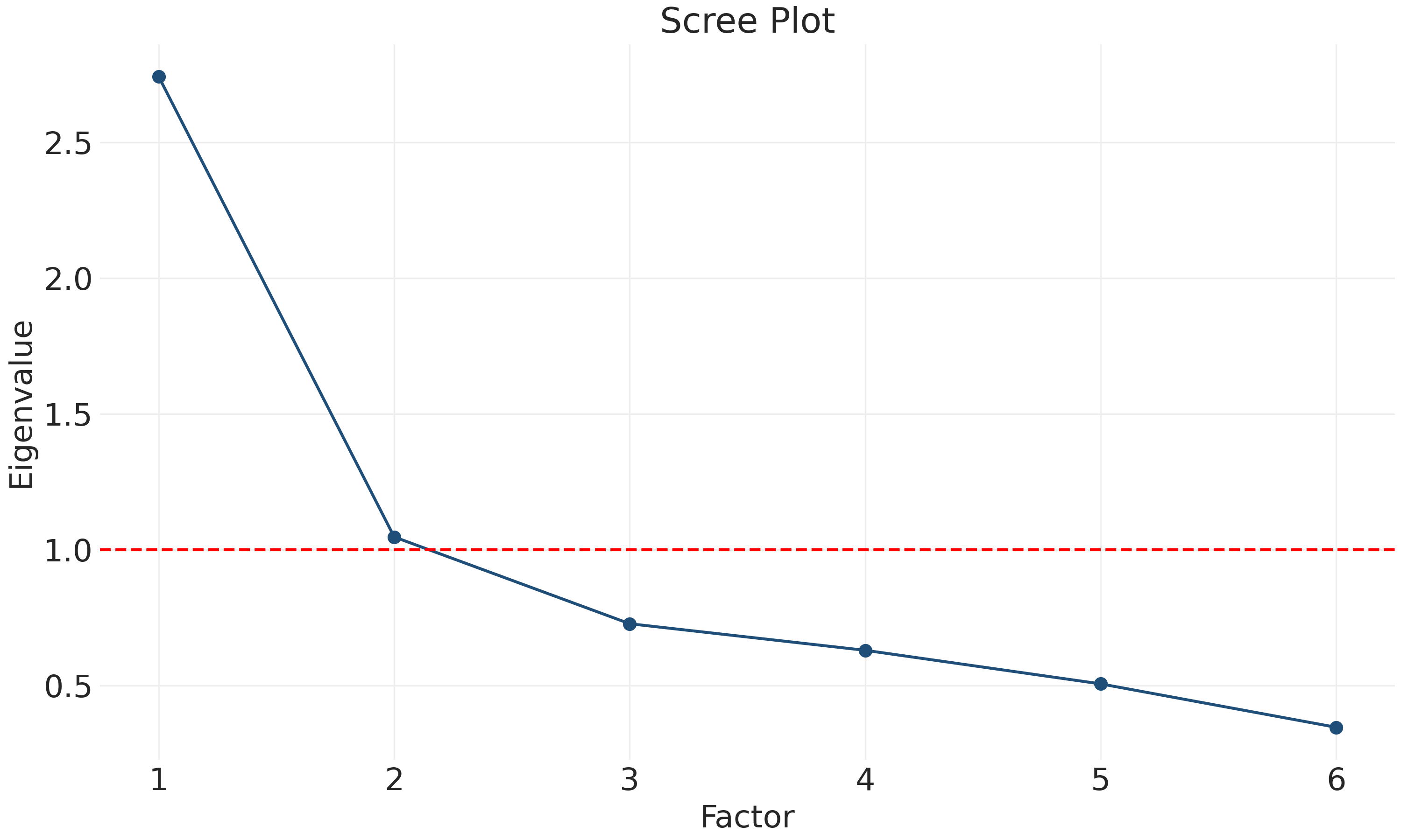
The plot shows a clear “elbow” after the first factor. Using the Kaiser criterion (eigenvalue > 1), we see that Factor 1 has an eigenvalue of approximately 2.7 (well above 1) and Factor 2 is borderline at approximately 1.0. Factors 3-6 all fall well below 1.
However, we should be cautious about mechanistically applying the eigenvalue > 1 rule. As noted above, there’s no strong theoretical justification for requiring factors to explain more variance than a single item. The borderline eigenvalue for Factor 2 (approximately 1.0) suggests we should examine factor loadings and substantive interpretation rather than relying solely on this mechanical rule. The visual “elbow” in the scree plot provides additional evidence for a one-factor solution, but the decision should ultimately consider multiple sources of evidence.
The sharp drop after Factor 1 and the dominant first eigenvalue suggest that one primary factor underlies these six items, which aligns with our Cronbach’s \(\alpha\) = 0.704 (borderline reliability). However, as we saw in the correlation heatmap, populism_6 shows near-zero correlations with other items, suggesting it measures a different construct. The borderline eigenvalue for Factor 2 (approximately 1.0) and the poor performance of populism_6 suggest we should examine factor loadings to identify problematic items.
One potential explanation for the unidimensional structure is that we have an unequal number of indicators per theoretical dimension. The anti-elite dimension has three items (populism_3, populism_4, populism_8), while the popular sovereignty and homogenous will dimensions each have only one item (populism_7 and populism_2, respectively). When one dimension is better measured with multiple indicators, it can dominate the factor structure, making it difficult for less-well-measured dimensions to emerge as separate factors. This doesn’t necessarily mean the multidimensional theory is wrong, it may simply reflect measurement limitations in our item battery.
However, the more immediate issue is that populism_6 appears to measure authoritarianism rather than populism, as evidenced by its near-zero correlations with other items. We’ll examine this more closely by re-running the analysis excluding populism_6.
If you were wondering, the negative factor loadings are fine. In factor analysis, the sign of factors is arbitrary. What matters is that items load consistently. All items (except populism_6) have moderate to strong loadings in the same direction.
8.2.5.3 Factor Loadings, excluding populism_6
Let’s examine how each item loads onto the primary factor after excluding the problematic populism_6 item:
# Exclude `populism_6` from the analysis
X_refined = X.drop(columns=["pes21_populism_6"])

print(f"Refined scale items: {X_refined.columns.tolist()}")
print(f"Number of items in refined scale: {len(X_refined.columns)}")

# Recalculate Cronbach's alpha for the refined scale
alpha_refined = pg.cronbach_alpha(data=X_refined)
print(f"\nCronbach's $\alpha$ (refined scale, excluding `populism_6`) = {alpha_refined[0]:.3f}")

# Fit a one-factor model on refined data
fa_one_factor = FactorAnalyzer(n_factors=1, rotation=None)
fa_one_factor.fit(X_refined.dropna())

# Get factor loadings
loadings = fa_one_factor.loadings_

# Create a dataframe for easier viewing
loadings_df = pd.DataFrame(loadings, index=X_refined.columns, columns=["Factor 1"])
loadings_df = loadings_df.round(3)
loadings_df
After removing populism_6, Cronbach’s \(\alpha\) increases from 0.704 to 0.791. All five remaining items have factor loadings exceeding |0.5|: populism_3 (-0.843), populism_8 (-0.748), populism_4 (-0.631), populism_2 (-0.556), and populism_7 (-0.514). Again, the negative signs are arbitrary in factor analysis; what matters is that all items load consistently on the same factor.
# Visualize the loadings
plt.figure(figsize=(8, 6))
plt.barh(range(len(loadings_df)), loadings_df["Factor 1"].abs(), alpha=0.85)

plt.yticks(
    range(len(loadings_df)), [n.replace("pes21_", "") for n in loadings_df.index]
)
plt.xlabel("Factor Loading (Absolute Values)")
plt.title("Factor Loadings on Primary Populism Factor")
plt.axvline(
    x=0.3, color="r", linestyle="--", alpha=1, linewidth=3, label="Weak threshold (0.3)"
)
plt.axvline(
    x=0.5,
    color="orange",
    linestyle="--",
    alpha=1,
    linewidth=3,
    label="Moderate threshold (0.5)",
)
plt.legend(loc="lower center", bbox_to_anchor=(0.5, -0.25), ncol=2)
plt.tight_layout()
The results show substantial improvement after excluding populism_6. Cronbach’s \(\alpha\) increased from 0.704 to 0.791, moving from “acceptable” to “good” reliability. This improvement provides strong evidence that populism_6 (“strong leader even if bends rules”) measures a different construct than the other items. All factor loadings are now moderate to strong, with every item loading above |0.5|, indicating they all contribute meaningfully to the underlying populism factor.
Populism_3 (politicians don’t care) has the strongest loading at -0.843, followed by populism_8 (care only about rich/powerful) at -0.748, populism_4 (politicians trustworthy - reversed) at -0.631, populism_2 (compromise = selling out) at -0.556, and populism_7 (people should decide) at -0.514.
# Calculate communalities (proportion of variance in each item explained by the factor)
communalities = fa_one_factor.get_communalities()
communalities_df = pd.DataFrame(
    {
        "Item": X_refined.columns,
        "Communality": communalities,
        "Unique Variance": 1 - communalities,
    }
)
communalities_df = communalities_df.round(3)
communalities_df
Communalities also improved, with items like populism_3 (71%) and populism_8 (56%) showing substantial variance explained by the common factor, indicating they are excellent indicators of the underlying construct.
Again, negative signs on the loadings are not a problem. In factor analysis, the direction (sign) of factors is arbitrary. What matters is that all items load consistently in the same direction, which they do. The negative loadings simply mean the factor is oriented in the opposite direction, but all items still measure the same underlying construct.
8.2.5.3.1 Examining Multiple Factors
Although we found evidence for a single dominant factor, let’s examine how items load on the first three factors to better understand the structure and see whether the theoretical dimensions we discussed earlier emerge:
# Fit a three-factor model on refined data
fa_three_factor = FactorAnalyzer(n_factors=3, rotation='varimax')
fa_three_factor.fit(X_refined.dropna())

# Get eigenvalues and variance explained
ev_three, v_three = fa_three_factor.get_eigenvalues()
variance_explained = ev_three / ev_three.sum() * 100

# Get factor loadings
loadings_three = fa_three_factor.loadings_

# Create a dataframe for easier viewing
loadings_three_df = pd.DataFrame(
    loadings_three,
    index=X_refined.columns,
    columns=[f"Factor {i+1}" for i in range(3)]
)
loadings_three_df = loadings_three_df.round(3)

print("Factor Loadings (Three-Factor Model with Varimax Rotation):")
print(loadings_three_df)
print(f"\nVariance Explained:")
for i in range(3):
    print(f"Factor {i+1}: {variance_explained[i]:.1f}% (eigenvalue = {ev_three[i]:.2f})")
# Visualize the loadings on all three factors
fig, axes = plt.subplots(1, 3, figsize=(18, 6))
# Get the consistent ordering (lowest PI to highest) from the item names
ordered_idx = sorted(
X_refined.columns, key=lambda n: n.replace("pes21_populism_", "PI ")
)
ordered_names = [n.replace("pes21_populism_", "PI ") for n in ordered_idx]
for i, ax in enumerate(axes):
factor_num = i + 1
sorted_loadings = loadings_three_df.loc[ordered_idx, f"Factor {factor_num}"]
colors = ["red" if x < 0 else "steelblue" for x in sorted_loadings.values]
ax.barh(
range(len(sorted_loadings)), sorted_loadings.values, color=colors, alpha=0.7
)
ax.set_yticks(range(len(sorted_loadings)))
ax.set_yticklabels(ordered_names)
ax.set_xlabel("Factor Loading")
ax.set_title(
f"Factor {factor_num}\n({variance_explained[i]:.1f}% variance, λ={ev_three[i]:.2f})"
)
ax.axvline(x=0, color="black", linestyle="-", linewidth=0.5)
ax.axvline(x=0.3, color="red", linestyle="--", alpha=0.5, linewidth=1)
ax.axvline(x=0.5, color="orange", linestyle="--", alpha=0.5, linewidth=1)
ax.grid(True, alpha=0.3, axis="x")
plt.tight_layout()The three-factor solution shows that Factor 1 dominates, explaining most of the variance. Factors 2 and 3 have much smaller eigenvalues and explain little variance. This confirms our earlier finding: despite populism’s theoretical multidimensionality, these five CES items form a coherent unidimensional scale.
The three theoretical dimensions (anti-elite, popular sovereignty, homogenous will) do not emerge as separate factors in the 2021 CES data. We can proceed on the notion that the refined 5-item scale (excluding populism_6, that is) provides a reliable measure of populism (\(\alpha\) = 0.791) with a clear single-factor structure.
Factor loadings (or component loadings) tell us how strongly each item relates to the underlying factor. They’re properties of the variables/survey items, not the respondents. Loadings help us understand which items are good indicators of the latent construct and which should be excluded.
Factor scores (or PCA scores), on the other hand, combine each person’s responses across all items into a single value. Loadings tell us the weights to use when combining items, but scores tell us where each person falls on the populism dimension. In practice, researchers report loadings to demonstrate measurement validity (showing that items load strongly on the factor), but use scores as the actual measure in subsequent analyses.
You might wonder: why not just use factor scores from factor analysis instead of switching to PCA? This is a valid question that requires careful attention to what these methods actually do.
PCA is a descriptive data-reduction method that finds linear combinations of variables maximizing variance. It’s a mathematical transformation of the data with no probabilistic model. PCA rotates the variable space to create new axes (principal components) that capture maximum variance, but it doesn’t model latent variables or measurement error.
Common factor analysis is a latent variable model that specifies how observed variables are generated by unobserved factors plus measurement error (\(\mathbf{X} = \mathbf{\Lambda}\boldsymbol{\eta} + \boldsymbol{\epsilon}\)). This is a generative model regardless of whether estimation is done using Frequentist methods (maximum likelihood) or Bayesian methods (posterior distributions). The model assumes latent factors cause observed covariances, making it appropriate for measurement theory.
We use factor analysis to understand measurement structure—examining how items relate to latent dimensions, identifying problematic items through factor loadings, and evaluating dimensionality. But we use PCA to produce the final populism index because: (1) it’s the approach used in published CES research (Wu & Dawson 2024), ensuring comparability; (2) when there’s one dominant factor (as we have), FA scores and PCA scores are nearly identical; and (3) PCA scoring is computationally simpler. The choice is partly conventional (aligning with published work) and partly pragmatic, but both approaches produce substantively similar results when the measurement structure is clear.
8.2.6 Principal Component Analysis
At this point, I’m going to say something that might really piss you off: having done all that, we’re going to set the factor analysis aside and do our measurements using an entirely different tool, Principal Component Analysis (PCA). Among other things, the PCA will generate a set of scores on a populism index that we can apply to our survey respondents.
But why did we go through all that factor analysis if we’re just going to use PCA for the final index? This is a fair question that gets at an important methodological issue.
The distinction between factor analysis (which models measurement error explicitly) and PCA (which doesn’t) matters primarily in inferential contexts where you want to quantify uncertainty about latent structure and make population-level inferences. In such cases, a Bayesian generative approach would be ideal—treating latent factors as part of a probabilistic data-generating process with explicit uncertainty quantification through posterior distributions.
But we’re doing descriptive measurement here, not formal inference. We’re summarizing patterns in observed data to create a populism index, not making probabilistic claims about population parameters. For this purpose, PCA is perfectly adequate and widely used. We could have done this entire analysis using only PCA—examining PCA component loadings, creating scree plots from PCA, and generating PCA scores. This would be simpler and equally valid.
So why include factor analysis at all? Two reasons. First, factor analysis provides standard diagnostic tools (KMO, Bartlett’s test, factor loadings, communalities) that are widely used in published research to evaluate measurement quality. Understanding these tools helps you engage with the broader literature. Second, the conceptual framework of factor analysis—latent factors causing observed covariances—aligns with measurement theory even when we ultimately use PCA for scoring. Factor analysis helps us think about measurement structure, even if PCA does the final calculations.
The practical reality: when items are highly correlated and form a clear single factor (as ours do after removing populism_6), factor analysis and PCA produce nearly identical results. The theoretical distinction matters more for inference than for descriptive measurement.
Wu and Dawson (2024) explicitly describe their operationalization: they “standardized the five items and extracted the first principal component” as their populism measure. Let’s replicate this approach:
from sklearn.decomposition import PCA

# Get complete cases for PCA
X_complete = ces[X_refined.columns].dropna()

# Standardize the items (as published research does)
X_standardized = (X_complete - X_complete.mean()) / X_complete.std()

# Extract first principal component
pca = PCA(n_components=1)
pca_scores = pca.fit_transform(X_standardized)

# Add PCA scores back to the main dataframe
# Initialize with NaN
ces["populism_index_pca"] = np.nan
# Fill in the scores for complete cases
ces.loc[X_complete.index, "populism_index_pca"] = pca_scores.flatten()

# Show variance explained
print(
    f"\nVariance explained by first principal component: {pca.explained_variance_ratio_[0]:.3f}"
)
print("Published research reports ~55% variance explained")

# Show component loadings
loadings_pca = pd.DataFrame(
    {
        "Item": X_refined.columns,
        "PC1 Loading": pca.components_[0],
    }
)
loadings_pca["Abs Loading"] = loadings_pca["PC1 Loading"].abs()
loadings_pca = loadings_pca.sort_values("Abs Loading", ascending=False)
print("\nPrincipal Component Loadings:")
print(loadings_pca.round(3))

# Descriptive statistics for PCA-based index
print("\nPCA-Based Populism Index Descriptive Statistics:")
print(ces["populism_index_pca"].describe())
The first principal component explains 54.9% of variance, aligned with published research using this battery. Component loadings range from 0.512 (populism_3) to 0.383 (populism_7). The PCA-based index is standardized with mean ≈ 0 and SD = 1.66.
8.2.7 Mean-based vs. PCA-based Populism Indices
We’ve now created two different populism indices: a simple mean-based index and a PCA-based index. Both measure the same underlying construct but with different properties. Let’s compare them to understand their similarities and differences.
# Correlation between the two indices
corr = ces[["populism_index_mean", "populism_index_pca"]].corr().iloc[0, 1]
print(f"Correlation between mean-based and PCA-based indices: {corr:.3f}")

# The correlation should be very high (typically > 0.95)
# Use the PCA-based index for subsequent analyses to align with published research
ces["populism_index"] = ces["populism_index_pca"]
The correlation between mean-based and PCA-based indices is 0.999.
Let’s visualize the distribution of our populism index:
fig, axes = plt.subplots(1, 2, figsize=(14, 5))

# Left panel: Mean-based index
ax1 = axes[0]
mean_data = ces["populism_index_mean"].dropna()
# Use pd.cut to create equal-width bins, then count
n_bins = 20
bins_mean = pd.cut(mean_data, bins=n_bins)
counts_mean = bins_mean.value_counts().sort_index()
bin_centers_mean = [interval.mid for interval in counts_mean.index]
bin_width_mean = counts_mean.index[0].length

ax1.bar(
    bin_centers_mean,
    counts_mean.values,
    width=bin_width_mean * 0.9,
    edgecolor="black",
    alpha=0.7,
)
ax1.axvline(
    mean_data.mean(),
    color="red",
    linestyle="--",
    linewidth=2,
    label=f"Mean = {mean_data.mean():.2f}",
)
ax1.set_xlabel("Populism Index\n(mean of 5 Likert items, each 1-5)")
ax1.set_ylabel("Frequency")
ax1.set_title("Mean-Based Populism Index")
ax1.legend()
ax1.grid(True, alpha=0.3)

# Right panel: PCA-based index
ax2 = axes[1]
pca_data = ces["populism_index_pca"].dropna()
# Use pd.cut to create equal-width bins, then count
bins_pca = pd.cut(pca_data, bins=n_bins)
counts_pca = bins_pca.value_counts().sort_index()
bin_centers_pca = [interval.mid for interval in counts_pca.index]
bin_width_pca = counts_pca.index[0].length

ax2.bar(
    bin_centers_pca,
    counts_pca.values,
    width=bin_width_pca * 0.9,
    edgecolor="black",
    alpha=0.7,
)
ax2.axvline(
    pca_data.mean(),
    color="red",
    linestyle="--",
    linewidth=2,
    label=f"Mean = {pca_data.mean():.2f}",
)
ax2.set_xlabel("Populism Index\n(standardized PC scores)")
ax2.set_ylabel("Frequency")
ax2.set_title("PCA-Based Populism Index")
ax2.legend()
ax2.grid(True, alpha=0.3)

plt.tight_layout()
The mean-based populism index is the simple average of the five Likert items, each ranging from 1-5, so the index ranges from 1 (low populism) to 5 (high populism). The PCA-based populism index produces standardized scores (mean ≈ 0, SD ≈ 1.66) where higher values indicate stronger populist attitudes. Both capture the same underlying construct but have different scaling—the mean-based index preserves the original 1-5 scale, while the PCA-based index is standardized around zero.
For the remainder of this chapter, and the next on regression, we’ll use the PCA-based index (populism_index) as our primary measure, consistent with published research using the 2021 CES populism battery (wu2024?; medeiros2023?; qmcpe2023?).
8.2.8 A Generative Perspective: Bayesian Factor Analysis
We’ve checked the standard diagnostic boxes: Bartlett’s test is “significant,” KMO is in the excellent range, the scree plot shows a clear elbow, and our factor loadings are strong. These Frequentist diagnostics support using these items as a populism scale. But there are more principled ways to think about this measurement problem.
A Bayesian factor analysis would treat this as a generative measurement model, explicitly modeling how latent populist attitudes produce observed survey responses. Instead of descriptive diagnostics, we’d specify:
\[ \mathbf{y}_i = \boldsymbol{\Lambda} \boldsymbol{\eta}_i + \boldsymbol{\epsilon}_i \]
where \(\mathbf{y}_i\) is person \(i\)’s vector of observed item responses, \(\boldsymbol{\eta}_i\) is their latent populism score(s), \(\boldsymbol{\Lambda}\) is the matrix of factor loadings (how strongly each item relates to the latent factor), and \(\boldsymbol{\epsilon}_i\) is measurement error. Each component gets a prior distribution:
Factor loadings (\(\boldsymbol{\Lambda}\)): How strongly does each item indicate populism? We might use weakly informative priors like \(\lambda_j \sim \text{Normal}(0, 1)\) or incorporate theory-based expectations about which items should load more strongly.
Latent scores (\(\boldsymbol{\eta}_i\)): Each person’s unobserved populism level, typically \(\eta_i \sim \text{Normal}(0, 1)\) for identification.
Measurement error (\(\boldsymbol{\epsilon}_i\)): Item-specific error variances, perhaps \(\epsilon_j \sim \text{Normal}(0, \sigma^2_j)\) with priors on \(\sigma^2_j\).
With this model specified, Bayesian inference produces posterior distributions for all parameters. Instead of point estimates of factor loadings, we get full uncertainty distributions. Instead of a single “number of factors” decision based on eigenvalues > 1, we’d compare models with different numbers of factors using posterior predictive checks and information criteria (WAIC, LOO).
The Bayesian approach asks different questions than Frequentist diagnostics:
Does a 1-factor model reproduce the covariance structure? Check via posterior predictive checks comparing observed and model-implied correlation matrices.
Does a 2-factor or 3-factor model fit better? Compare using WAIC or leave-one-out cross-validation, which balance fit and complexity.
How certain are we about dimensionality? Examine how posterior predictive performance changes across models with different numbers of factors.
How much measurement uncertainty exists? Posterior distributions for factor loadings and latent scores quantify this directly.
Which items are reliable indicators? Examine posterior distributions of factor loadings—items with loadings confidently away from zero are strong indicators.
In a Bayesian workflow, tools like scree plots remain useful for building intuition and informing priors, but they don’t make final decisions. The model comparison framework provides a principled way to evaluate competing structures while quantifying uncertainty throughout.
Why didn’t we implement Bayesian factor analysis here? Two reasons. First, pedagogically, we’re building toward Bayesian inference gradually—this chapter focuses on measurement concepts and introduces factor analysis descriptively before we tackle full Bayesian latent variable models. Second, practically, when measurement structure is clear (as ours is with one dominant factor), descriptive factor analysis and PCA produce substantively similar results to Bayesian approaches for index construction. The Bayesian approach would add uncertainty quantification and formal model comparison, which matter more for inference than for descriptive measurement.
For researchers working with complex measurement structures, ambiguous dimensionality, or who need formal inference about latent variables, Bayesian factor analysis (or more generally, Bayesian structural equation modeling) provides a principled framework. For our purposes—creating a populism index to use in subsequent analyses—the descriptive approach suffices, especially since it aligns with published CES research.
8.2.9 The “Populism Index”
Now that we’ve created our PCA-based populism index, let’s examine its distribution and explore how it relates to other variables. This will help us understand what the index captures and set up analyses for the next chapter on regression.
# Distribution of the populism index
fig, axes = plt.subplots(1, 2, figsize=(14, 5))

# Left: Histogram with density overlay
ax1 = axes[0]
pop_data = ces["populism_index"].dropna()
ax1.hist(pop_data, bins=30, density=True, alpha=0.7, edgecolor="black")
ax1.axvline(
    pop_data.mean(),
    color="red",
    linestyle="--",
    linewidth=2,
    label=f"Mean = {pop_data.mean():.2f}",
)
ax1.axvline(
    pop_data.median(),
    color="blue",
    linestyle="--",
    linewidth=2,
    label=f"Median = {pop_data.median():.2f}",
)
ax1.set_xlabel("Populism Index (PCA-based)")
ax1.set_ylabel("Density")
ax1.set_title("Distribution of Populism Index")
ax1.legend()
ax1.grid(True, alpha=0.3)

# Right: Box plot
ax2 = axes[1]
ax2.boxplot(
    pop_data,
    vert=True,
    patch_artist=True,
    boxprops=dict(facecolor="steelblue", alpha=0.7),
)
ax2.set_ylabel("Populism Index (PCA-based)")
ax2.set_title("Box Plot of Populism Index")
ax2.grid(True, alpha=0.3, axis="y")

plt.tight_layout()
plt.savefig("_figures/populism_index_distribution.png", dpi=300)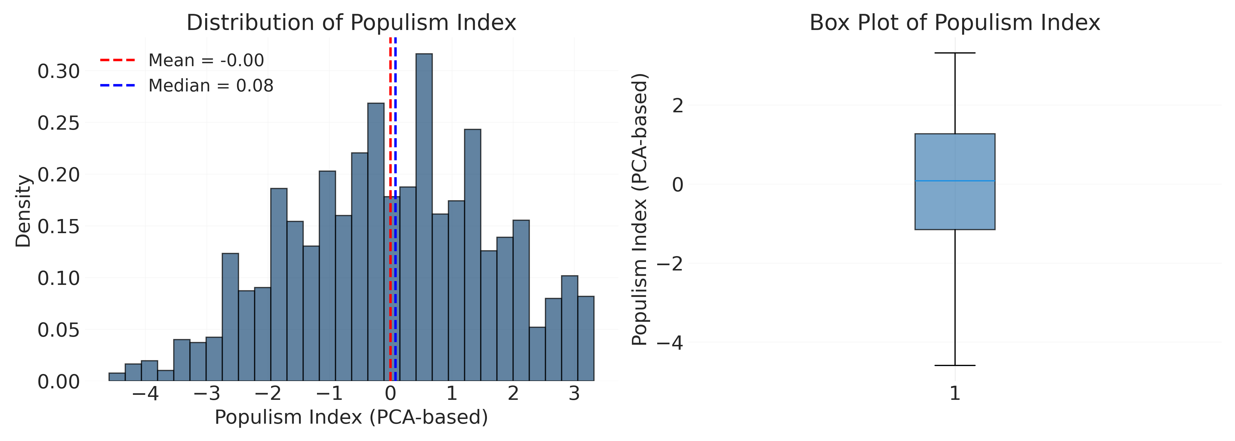
The populism index shows a roughly symmetric distribution centered near zero, which is expected since PCA scores are standardized. Most respondents fall within ±2 standard deviations, with relatively few extreme values. This suggests populist attitudes are distributed across the population rather than concentrated in a small subset.
Let’s quickly check how populism relates to education to prime ourselves for upcoming content on regression. In short, we would expect higher populism among those with lower education.
if "cps21_education" in ces.columns:
    edu_pop = ces[["cps21_education", "populism_index"]].dropna()

    edu_pop["edu_group"] = pd.cut(edu_pop["cps21_education"],
                                   bins=[0, 3, 6, 10],
                                   labels=["Low", "Medium", "High"])

    fig, ax = plt.subplots(figsize=(10, 6))

    edu_groups = ["Low", "Medium", "High"]
    data_by_group = [edu_pop[edu_pop["edu_group"] == g]["populism_index"].dropna()
                     for g in edu_groups]

    bp = ax.boxplot(data_by_group, labels=edu_groups, patch_artist=True,
                    boxprops=dict(facecolor="steelblue", alpha=0.7))
    ax.set_xlabel("Education Level")
    ax.set_ylabel("Populism Index")
    ax.set_title("Populism Index by Education Level")
    ax.axhline(y=0, color="red", linestyle="--", alpha=0.5)
    ax.grid(True, alpha=0.3, axis="y")

    plt.tight_layout()
    plt.savefig("_figures/populism_by_education.png", dpi=300)
8.3 Conclusion
Many concepts we care about in social science like populism, trust, and political polarization cannot be directly observed. Instead, we measure them through multiple observable indicators and infer the underlying latent structure from patterns in the data. The populism index we created here will be used in the next chapter on regression, where we’ll examine what predicts populist attitudes and how populism relates to other political outcomes. The work we’ve done here (examining correlations, assessing reliability, identifying problematic items, and creating a validated scale) provide a solid measurement foundation for the next analysis. Thinking generatively about how latent constructs might produce patterns in observed data helps whether we use descriptive tools like PCA or generative models like Bayesian factor analysis.