import yaml
import numpy as np
import pandas as pd
import matplotlib.pyplot as plt
import seaborn as snsBy the end of this chapter, you will be able to:
- Define what statistical association means and illustrate it using both numerical and categorical variables.
- Use correlation as a measure of association for numerical data, and interpret the strength and direction of linear relationships between variables.
- Create and interpret contingency tables (crosstabs) using proportion and percentage calculations to assess relationships between categorical variables.
- Compute and interpret Pearson correlation coefficients for pairs of variables and understand correlation matrices as summaries of associations across multiple variables.
- Visualize associations by constructing and interpreting heatmaps for joint distributions (such as crosstabs) and correlation matrices.
- Understand and evaluate the measurement challenges involved in using correlation with ordinal (Likert-type) survey data, including considerations for appropriate analysis.
- Discuss the rationale and design of Likert-style survey items, and make informed decisions about recoding response options such as “Don’t know” or “Prefer not to answer.”
7.1 Introduction
Association is the foundation of quantitative social science. Nearly every research question we ask involves understanding how variables relate to one another: Do people with more education earn higher incomes? Does partisan identity predict attitudes toward climate policy? Are citizens’ beliefs organized into coherent ideological systems?
This chapter introduces the logic of association, how we measure, visualize, and interpret relationships between variables. We’ll work with two types of data that require different analytical approaches:
- Categorical variables (like partisan identity or survey response categories), where we use contingency tables and heatmaps to examine how categories co-occur
- Numeric or quasi-numeric variables (like Likert-scale attitude items), where we use correlation to measure the strength and direction of linear relationships
We’ll build from simple pairwise associations to more complex questions about how political attitudes are organized in mass publics. Throughout, we’ll work with Canadian Election Study (CES) 2021 data, examining how Canadians’ political identities, attitudes toward inequality, environmental policy, immigration, and other issues connect to one another.
By the end of this chapter, you’ll understand not just how to calculate measures of association, but what they mean and when to use them.
7.1.1 Setup
We’ll use a config file (data/ces21.yaml, which Python will download using the link in the code block below) containing metadata for the CES 2021 dataset, including variable labels and response category mappings, URLs for downloading processed data, question text for survey items, groupings of related variables (e.g., all Likert items, demographic variables), and so on. This structure keeps our code clean by separating data documentation from analysis code. We’ll use it throughout to map numeric codes (1, 2, 3…) to readable labels (“Liberal”, “Conservative”, “NDP”…).
import requests

# ↓ downloads a config file
config_url = "http://bit.ly/4nLXr2y"
response = requests.get(config_url)
response.raise_for_status()
ces21_qs = yaml.safe_load(response.text)

# ↓ downloads data and loads into a DataFrame
data_url = ces21_qs.get("data_urls").get("ces2021_cleaned")
ces = pd.read_parquet(data_url)
We’ll create two filters for our dataset. The first, valid_data, will select all respondents who provided valid data on either the campaign period survey (cps21_data_quality == 0) or the post-election survey (pes21_data_quality == 0). This filter allows us to access a wider range of opinion variables, since most respondents completed both surveys, allowing us to link question sets from both surveys. The second filter, both_surveys_valid, is more restrictive: it includes only respondents with valid data from both surveys (cps21_data_quality == 0 and pes21_data_quality == 0). We’ll use both_surveys_valid to compare a question related to partisan identity, but otherwise we’ll use the more inclusive filter.
# (quality == 0 means valid data)
valid_data = ces[
    (ces["cps21_data_quality"] == 0) | (ces["pes21_data_quality"] == 0)
].copy()

# For analyses requiring both surveys, create separate filter
both_surveys_valid = ces[
    (ces["cps21_data_quality"] == 0) & (ces["pes21_data_quality"] == 0)
].copy()

# Use valid_data for main analysis (post-election survey focus)
pes = valid_data.copy()
pes.info()
# Helper functions for table creation
def freq_table_with_pct(series, mapping=None, label_col="Response"):
"""Create frequency table with counts and percentages."""
df = series.value_counts(dropna=False).sort_index().to_frame("Count")
df.index.name = None
if mapping:
df[label_col] = df.index.map(mapping).fillna("")
total = df["Count"].sum()
df["N (%)"] = df["Count"].apply(lambda n: f"{int(n):,} ({n/total*100:.1f}%)")
return df[[label_col, "N (%)"]] if mapping else df[["N (%)"]]
def format_crosstab_with_pct(counts, pcts, row_labels=None, col_labels=None):
"""Format crosstab with 'N (%)' format using vectorized operations."""
combined = counts.copy().astype(object)
# Vectorized formatting - iterate but use vectorized operations where possible
for i in counts.index:
for j in counts.columns:
n = counts.loc[i, j]
if n > 0:
pct = pcts.loc[i, j]
combined.loc[i, j] = f"{int(n):,} ({pct*100:.1f}%)"
else:
combined.loc[i, j] = ""
if row_labels:
combined.index = combined.index.map(row_labels)
if col_labels:
combined.columns = combined.columns.map(col_labels)
combined.index.name = None
combined.columns.name = None
return combined
def format_crosstab_with_margins(counts, pcts, total_N, row_labels=None):
"""Format crosstab with margins, handling 'All' row/column specially."""
combined = counts.copy().astype(object)
# Format data rows (excluding "All" row)
data_rows = [idx for idx in counts.index if idx != "All"]
data_cols = [col for col in counts.columns if col != "All"]
for i in data_rows:
for j in data_cols:
n = counts.loc[i, j]
pct = pcts.loc[i, j]
combined.loc[i, j] = f"{int(n):,} ({pct:.1f}%)"
# Format "All" column with row percentage of total
n_all = counts.loc[i, "All"]
pct_row_all = (n_all / total_N) * 100
combined.loc[i, "All"] = f"{int(n_all):,} ({pct_row_all:.1f}%)"
# Format total row
for j in data_cols:
n = counts.loc["All", j]
pct = (n / total_N) * 100
combined.loc["All", j] = f"{int(n):,} ({pct:.1f}%)"
combined.loc["All", "All"] = f"{int(total_N):,}"
if row_labels:
combined.index = combined.index.map(row_labels)
combined.columns.name = None
combined.index.name = None
return combined7.2 Association
Most of what we’ve done so far has focused on frequency distributions when reporting raw counts, or relative frequency distributions when reporting percentages or proportions.1 For example, Table 7.1 reports the relative frequency distribution for pes21_inequal (“Is income inequality a big problem in Canada?”).
1 You might also see these referred to as marginal distributions, meaning the distribution of a single variable ignoring (i.e., summing/collapsing/marginalizing over) all others.
# Create frequency table with counts and percentages
income_inequality_mapping = ces21_qs.get("income_inequality_mapping")
inequality_attitudes = freq_table_with_pct(
    pes["pes21_inequal"],
    income_inequality_mapping,
    label_col="Response"
)
inequality_attitudes.to_markdown("_tables/income_inequality.md")
inequality_attitudes| Response | N (%) | |
|---|---|---|
| 1 | Definitely yes | 4,995 (26.3%) |
| 2 | Probably yes | 5,178 (27.2%) |
| 3 | Not sure | 1,754 (9.2%) |
| 4 | Probably not | 1,125 (5.9%) |
| 5 | Definitely not | 346 (1.8%) |
| 6 | DK/PNA | 355 (1.9%) |
| nan | 5,256 (27.7%) |
It’s clear from Table 7.1 alone that most respondents see income inequality as a big problem, but how would this distribution look if the responses were contingent on some other variable, such as partisan identity?
7.2.1 Partisan Identity Stability Between Surveys
Before exploring how partisan identity associates with other attitudes, let’s first examine the stability of partisan identity itself. The CES 2021 includes both a campaign period survey (CPS) and post-election survey (PES). Some respondents completed both surveys, allowing us to examine whether their partisan identities remained stable or changed between the two time points.
This analysis introduces key concepts we’ll use throughout the chapter (contingency tables and conditional distributions) using a concrete example. As you work through this section, pay attention to how we compare percentages across groups to identify patterns. We’ll formalize these ideas in the next section when we define association more precisely.
# Get mappings from YAML - note these differ between surveys!
cps_pid_mapping = ces21_qs.get("partisan_identity_mapping_cps21_fed_id")
pes_pid_mapping = ces21_qs.get("partisan_identity_mapping")

# Filter to respondents in both surveys with valid partisan ID responses
both_surveys = both_surveys_valid[
    (both_surveys_valid["cps21_fed_id"].notna())
    & (both_surveys_valid["pes21_pidtrad"].notna())
].copy()

print(f"Respondents in both surveys with valid partisan IDs: {len(both_surveys):,}")
# Map the IDs to labels
both_surveys["cps_pid_label"] = both_surveys["cps21_fed_id"].map(cps_pid_mapping)
both_surveys["pes_pid_label"] = both_surveys["pes21_pidtrad"].map(pes_pid_mapping)
# Create a flag for whether partisan ID switched
both_surveys["pid_switched"] = (
both_surveys["cps_pid_label"] != both_surveys["pes_pid_label"]
)
# Summary statistics
n_total = len(both_surveys)
n_switched = both_surveys["pid_switched"].sum()
n_stable = n_total - n_switched
pct_switched = (n_switched / n_total) * 100
print(f"Partisan ID Stability:")
print(f" Stable: {n_stable:,} ({100-pct_switched:.1f}%)")
print(f" Switched: {n_switched:,} ({pct_switched:.1f}%)")# Create tables for stable identities and switches directly
stable = (
both_surveys[both_surveys["cps_pid_label"] == both_surveys["pes_pid_label"]]
.groupby("cps_pid_label")
.size()
.reset_index(name="count")
.rename(columns={"cps_pid_label": "Partisan ID"})
)
stable.to_markdown("_tables/stable_partisan_identities.md", index=False)
switches = (
both_surveys[both_surveys["cps_pid_label"] != both_surveys["pes_pid_label"]]
.groupby(["cps_pid_label", "pes_pid_label"])
.size()
.reset_index(name="count")
.sort_values("count", ascending=False)
.head(15)
)
switches[["cps_pid_label", "pes_pid_label", "count"]].to_markdown(
"_tables/top_15_partsan_switches.md", index=False
)| Partisan ID | count |
|---|---|
| Another party | 75 |
| Bloc Québécois | 903 |
| Conservative | 2506 |
| DK/PNA | 428 |
| Green | 212 |
| Liberal | 3389 |
| NDP | 1460 |
| None of these | 753 |
| cps_pid_label | pes_pid_label | count |
|---|---|---|
| Liberal | NDP | 165 |
| DK/PNA | None of these | 158 |
| None of these | DK/PNA | 142 |
| DK/PNA | Liberal | 125 |
| Liberal | DK/PNA | 115 |
| None of these | Liberal | 111 |
| NDP | Liberal | 105 |
| None of these | Conservative | 103 |
| Liberal | None of these | 101 |
| Conservative | None of these | 100 |
| Conservative | People’s Party | 98 |
| Another party | People’s Party | 94 |
| Conservative | Liberal | 91 |
| Liberal | Conservative | 90 |
| DK/PNA | NDP | 85 |
# Map strength of partisan identity for both surveys
# 1 = Very strongly, 2 = Fairly strongly, 3 = Not very strongly, 4 = DK/PNA
pid_strength_mapping = {
    1: "Very strongly",
    2: "Fairly strongly",
    3: "Not very strongly",
    4: "DK/PNA",
}

strength_order = list(pid_strength_mapping.values())

both_surveys["cps_strength_label"] = both_surveys["cps21_fed_id_str"].map(
    pid_strength_mapping
)
both_surveys["pes_strength_label"] = both_surveys["pes21_pidtradstrong"].map(
    pid_strength_mapping
)

# Filter to valid CPS strength responses for analysis
analysis_df = both_surveys[both_surveys["cps_strength_label"].notna()].copy()
print(f"Respondents with valid strength data: {len(analysis_df):,}")
# Create contingency table: switched vs CPS strength of partisan ID
ct = pd.crosstab(
analysis_df["pid_switched"], analysis_df["cps_strength_label"], margins=True
)
ct = ct.reindex(columns=strength_order + ["All"], fill_value=0)
# Calculate row percentages for non-total rows
ct_pct = (
pd.crosstab(
analysis_df["pid_switched"],
analysis_df["cps_strength_label"],
normalize="index",
)
* 100
)
ct_pct = ct_pct.reindex(columns=strength_order, fill_value=0)
# Format table with margins
total_N = ct.loc["All", "All"]
combined_ct = format_crosstab_with_margins(
ct, ct_pct, total_N,
row_labels={False: "Stable", True: "Switched", "All": "Total"}
)
combined_ct.to_markdown("_tables/pid_switching_by_cps_strength.md")
combined_ct| Very strongly | Fairly strongly | Not very strongly | DK/PNA | All | |
|---|---|---|---|---|---|
| Stable | 2,742 (32.1%) | 4,473 (52.3%) | 1,236 (14.5%) | 94 (1.1%) | 8,545 (82.7%) |
| Switched | 340 (19.0%) | 823 (46.1%) | 573 (32.1%) | 50 (2.8%) | 1,786 (17.3%) |
| Total | 3,082 (29.8%) | 5,296 (51.3%) | 1,809 (17.5%) | 144 (1.4%) | 10,331 |
Note
The numbers in each row of Table 7.4 are row percentages. This means that for each row—whether “Stable,” “Switched,” or “Total”—the percentages add up to 100% as you move across the columns (from “Very strongly” to “Not very strongly” and “DK/PNA”), not down the columns.
Here’s how to read the table:
Stable row: Of all people who kept the same party identification, what percent felt “Very strongly,” “Fairly strongly,” and so on during the 2019 CPS?
For example, 32.1% of stable partisans felt “Very strongly” identified.
52.3% felt “Fairly strongly.”
The remaining percentages reflect progressively weaker identification.
Switched row: Of all people who switched their partisan identity, what percent felt “Very strongly,” “Fairly strongly,” etc., during the CPS?
For instance, only 19.0% of switchers felt “Very strongly,” while 46.1% felt “Fairly strongly.”
Total row: Of all respondents, regardless of switching, what percentage felt each level of strength?
The key insight comes from comparing across these rows:
- People who felt “Very strongly” identified in the CPS were more likely to stay stable (32.1% among stable vs. 19.0% among switchers).
- People who felt “Not very strongly” were more likely to switch (32.1% among switchers vs. 14.5% among stable).
- This shows an association between strength of partisan identity and stability: respondents with weaker partisan identity are more likely to switch parties.
# Calculate partisan identity distribution in post-election survey
partisan_identity_mapping = ces21_qs.get("partisan_identity_mapping")

# Create frequency table, preserving party ordering
pid_counts = (
    pes["pes21_pidtrad"]
    .value_counts(dropna=False)
    .sort_index()
    .reindex(list(partisan_identity_mapping.keys()))
    .dropna()
)

pid_counts_perc_table = pd.DataFrame({
    "Parties": pid_counts.index.map(partisan_identity_mapping),
    "N (%)": pid_counts.apply(
        lambda n: f"{int(n):,} ({n/pid_counts.sum()*100:.1f}%)"
    )
})
pid_counts_perc_table.index.name = None

pid_counts_perc_table.to_markdown("_tables/pes21_pidtrad_mapped.md")
pid_counts_perc_table| Parties | N (%) | |
|---|---|---|
| 1 | Liberal | 4,214 (30.6%) |
| 2 | Conservative | 3,071 (22.3%) |
| 3 | NDP | 2,059 (15.0%) |
| 4 | Bloc Québécois | 1,227 (8.9%) |
| 5 | Green | 376 (2.7%) |
| 6 | People’s Party | 305 (2.2%) |
| 7 | Another party | 198 (1.4%) |
| 8 | None of these | 1,369 (10.0%) |
| 9 | DK/PNA | 934 (6.8%) |
Respondents are given a list of political parties and asked to identify party with which they most identify, if any. Table 7.5 breaks down the distribution of responses. We can see that the sample includes substantial representation from Canada’s three major federal parties: Liberals (30.2%), Conservatives (22.2%), and NDP (14.7%). The Bloc Québécois, which only runs candidates in Quebec, Greens, and People’s Party represent 8.6%, 2.5%, and 2.1% of the sample, respectively. The final category, DK/PNA (Don’t know / prefer not to answer), rounds out the distribution with 6.6%.
The partisan stability analysis above demonstrated a key pattern: respondents with stronger initial partisan identification were more likely to maintain that identity. This is an example of a systematic relationship between two variables, or association. When variables are associated, knowing someone’s value on one variable helps predict their value on the other.
Now let’s formalize what we mean by association and examine the tools for measuring it.
7.2.2 Contingency (Categorical Data)
In previous chapters, we described the distribution of quantitative variables such as “feeling thermometers” using measures of central tendency (mean, median, mode)2 and dispersion (variance, standard deviation).3 These summaries all assume variables containing numbers with meaningful distance between values, so we can’t meaningfully compute them when we’re working with categorical data. Instead, we summarize how often categories occur and how evenly responses are spread across categories.
2 Central tendency refers to measures that describe the “centre” or typical value of a dataset. The most common measures are the mean (arithmetic average), median (the middle value when ordered), and mode (the most frequently occurring value).
3 Dispersion refers to how spread out the data are, in other words how much the values differ from one another and from the typical value. If most observations are close together, we say a variable has low dispersion, and if the values are more scattered we say the variable has high dispersion. Two common measures of dispersion are variance (the average of the squared differences between each value and the mean), which captures how far, on average, the data points are from the mean, and standard deviation (the square root of the variance), which puts the measure back into the original units so it’s easier to interpret.
4 Proportions represent how much of a whole is represented by a part, typically as a number between 0 and 1 (e.g., 0.25 means 25 out of 100). Percentages are simply proportions multiplied by 100, expressing the same idea out of 100 (e.g., 25%). Both are useful for summarizing and comparing the relative frequency of categories in a dataset.
In short, when we have quantitative variables we think in terms of the variable’s centre and spread. When we have categorical data, we think in terms of the distribution of values across categories using proportions and percentages.4 Ordinal variables, such as strongly disagree \(\longrightarrow\) strongly agree, are categorical, but for reasons discussed below, we can think of them as an exception to the general rule.
A contingency table (or crosstab / crosstabulation) is a common way to display the relationship between two categorical variables. In such a table, the rows typically represent the possible values (or response categories) of one variable while the columns represent those of another variable. Each cell in the table then displays the frequency and/or percentage of observations that fall into the corresponding combination of the two variables.
7.2.2.1 Income Inequality Attitudes Contingent on Partisan Identity
To continue with our example, we might want to know how attitudes towards income inequality (e.g., “Is income inequality a big problem in Canada?”) vary according to a respondent’s partisan identity. WHY? WHAT DO WE EXPECT? WHAT THEORY? In this case, one dimension of the contingency table would list the possible responses to the income inequality question (such as “Definitely yes”, “Probably yes”, etc.), while the other would list the different partisan groups (e.g., Liberal, Conservative, NDP, etc.).
Constructing such a table lets us see the distribution of responses regarding income inequality for each political group, or equivalently which partisan groups are most likely to hold each attitude towards inequality. This joint distribution helps to reveal potential patterns of association between the two variables, such as whether people who identify with some parties are more likely to see inequality as a major problem than people who identify with other parties.
# Create crosstab showing income inequality attitudes by partisan identity
partisan_identity_mapping = ces21_qs.get("partisan_identity_mapping")
income_inequality_mapping = ces21_qs.get("income_inequality_mapping")

partisan_codes = list(partisan_identity_mapping.keys())
inequality_labels = list(income_inequality_mapping.values())

# Create mapped columns for crosstab
pes["pes21_inequal_mapped"] = pes["pes21_inequal"].map(income_inequality_mapping)

# Create crosstabs with counts and percentages, preserving order
ct_counts = pd.crosstab(pes["pes21_pidtrad"], pes["pes21_inequal_mapped"]).reindex(
    index=partisan_codes, columns=inequality_labels, fill_value=0
)
ct_perc = pd.crosstab(
    pes["pes21_pidtrad"], pes["pes21_inequal_mapped"], normalize="index"
).reindex(index=partisan_codes, columns=inequality_labels, fill_value=0)

# Format using helper function
combined = format_crosstab_with_pct(ct_counts, ct_perc)

# Add party labels as first column
combined.insert(0, "Parties", combined.index.map(partisan_identity_mapping))

combined.to_markdown("_tables/partisan_identity_x_inequal.md")
combined| Parties | Definitely yes | Probably yes | Not sure | Probably not | Definitely not | DK/PNA | |
|---|---|---|---|---|---|---|---|
| 1 | Liberal | 1,606 (38.1%) | 1,783 (42.3%) | 505 (12.0%) | 229 (5.4%) | 38 (0.9%) | 53 (1.3%) |
| 2 | Conservative | 566 (18.4%) | 1,114 (36.3%) | 546 (17.8%) | 600 (19.5%) | 194 (6.3%) | 51 (1.7%) |
| 3 | NDP | 1,241 (60.3%) | 625 (30.4%) | 120 (5.8%) | 39 (1.9%) | 6 (0.3%) | 28 (1.4%) |
| 4 | Bloc Québécois | 447 (36.4%) | 542 (44.2%) | 148 (12.1%) | 67 (5.5%) | 7 (0.6%) | 16 (1.3%) |
| 5 | Green | 186 (49.5%) | 131 (34.8%) | 37 (9.8%) | 14 (3.7%) | 4 (1.1%) | 4 (1.1%) |
| 6 | People’s Party | 64 (21.0%) | 89 (29.2%) | 51 (16.7%) | 57 (18.7%) | 39 (12.8%) | 5 (1.6%) |
| 7 | Another party | 68 (34.3%) | 70 (35.4%) | 24 (12.1%) | 15 (7.6%) | 16 (8.1%) | 5 (2.5%) |
| 8 | None of these | 554 (40.5%) | 462 (33.7%) | 181 (13.2%) | 82 (6.0%) | 31 (2.3%) | 59 (4.3%) |
| 9 | DK/PNA | 263 (28.2%) | 362 (38.8%) | 142 (15.2%) | 22 (2.4%) | 11 (1.2%) | 134 (14.3%) |
Tables and graphs lend themselves to different ends, even when they report the same information (see Few 2004; Healy and Moody 2014; Healy 2019). Tables such as these are primarily useful when we want to look up or compare specific numbers, such as responses provided by folks who identify with the populist People’s Party, whereas graphs are most useful when we need to understand structural patterns and relationships between numbers.
Figure 7.1 reports the information in Table 7.6 as a heatmap. Heatmaps encode a table of values into positions along a colour spectrum to make it easier to identify structural patterns in data, such as changes in scale, rate, or connection. Each cell in the heatmap represents a pair of values (one from the row and one from the column) with a colour gradient indicating how big the number is for that specific combination. Usually darker colours mean larger values and lighter colours mean smaller values, but this will always be indicated in the heatmaps “colourbar” legend (on the right of Figure 7.1, in this case).
plt.figure(figsize=(10, 6))

# Create version with party labels for visualization
ct_perc_labeled = ct_perc.copy()
ct_perc_labeled.index = ct_perc_labeled.index.map(partisan_identity_mapping)
ct_perc_pct = ct_perc_labeled * 100

annot_labels = ct_perc_pct.round(1).astype(str) + "%"

sns.heatmap(
    ct_perc_pct,
    annot=annot_labels,
    fmt="",
    cmap="YlGnBu",
    cbar_kws={"label": "Percentage (%)", "shrink": 0.8},
    linewidths=1,
)

# plt.title("Income Inequality Attitudes by Partisan Identity")
plt.xlabel("")
plt.ylabel("")
plt.xticks(rotation=0)
plt.tick_params(left=False, bottom=False)
plt.xticks(fontsize=12)
plt.yticks(fontsize=12)

plt.savefig(
    "_figures/income_inequality_partisan_identity.png", dpi=300, bbox_inches="tight"
)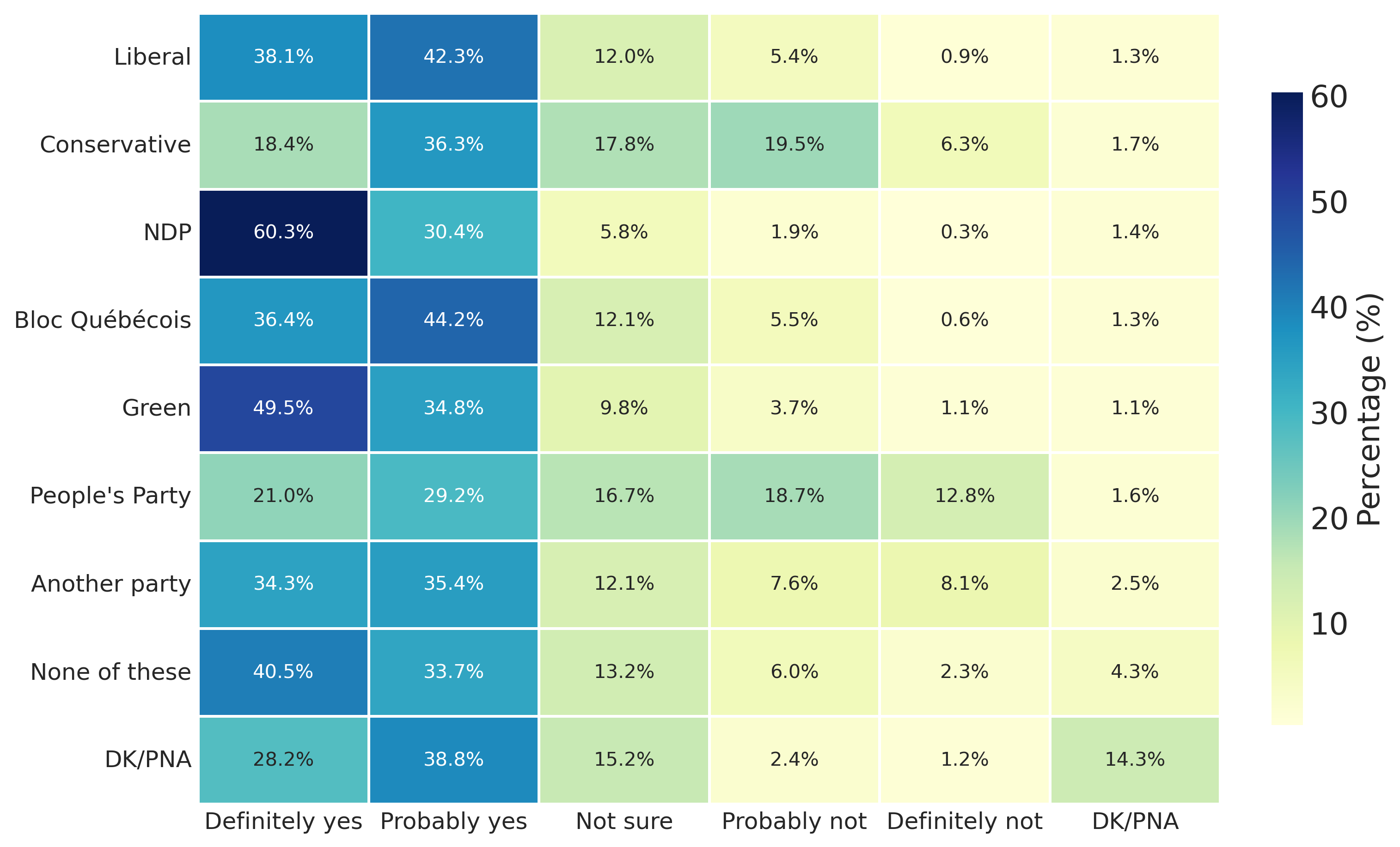
Contingency tables (e.g., Table 7.6) and heatmaps (e.g., Figure 7.1) report the number of cases that fall into each combination of categories across two categorical variables. They’re a simple but essential entry point into understanding the logic of association more generally.
If two variables are associated, it means that knowing someone’s category on one variable helps us predict their category on the other. For example, if there were no association between partisan identity and attitudes toward income inequality, then knowing someone’s partisan identity would tell us nothing useful about their attitude toward inequality. However, if these variables are associated, then knowing someone’s partisan identity would change our expectation of their attitude. This does not mean that one causes the other, of course, only that the two variables vary together in some systematic way.
We can gauge a potential association by examining the distribution of responses across rows or columns in a contingency table or heatmap. If the pattern of responses is similar across groups (e.g., if Liberals, Conservatives, and NDP supporters all show roughly the same distribution of attitudes), then it’s unlikely that there is an association between the variables. But if the pattern differs meaningfully across groups (e.g., if NDP supporters are much more likely to say inequality is a big problem than Conservative supporters), then there may be an association.
7.2.2.2 Interpreting Contingency Tables
To interpret contingency tables effectively, we need to understand three related concepts: joint distributions, marginal distributions, and conditional distributions.
The joint distribution refers to how often specific combinations of categories occur together (i.e., the counts in each cell of the table). For instance, in Table 7.6, one cell tells us how many Liberal identifiers said “Definitely yes” to the inequality question.
As noted earlier, the marginal distribution refers to the totals for each category of a single variable, ignoring the other variable. These are the row and column totals that would appear at the margins of the table. For example, the marginal distribution for partisan identity would show us the total number of respondents in each party category, regardless of their inequality attitudes.
The conditional distribution is perhaps most important for understanding association. It refers to the distribution of one variable within a specific category of another variable. In Table 7.6, we report row percentages, which show the conditional distribution of inequality attitudes within each partisan group. For instance, among Liberal identifiers, what percentage said “Definitely yes”? Among Conservatives, what percentage said the same?
To simplify things, we can interpret whether two categorical variables are associated by (1) looking at percentages within rows or columns to better understand conditional distributions and (2) comparing these conditional distributions across different groups, looking for meaningful differences. If the percentages are similar across groups, there is little or no association. If they differ substantially, there may be an association.
For example, looking at Table 7.6 and Figure 7.1, we can see that people identified with the NDP and Greens are much more likely to say inequality is “Definitely” a big problem (60.5% and 49.4%), especially compared to people identifying with the Conservatives and the People’s Party (18.2%, 21.4%).
Even with most responses in the “Definitely” and “Probably yes” categories for all identities, we can interpret this difference in conditional distributions as a likely association between partisan identity and their attitude towards income inequality. In other words, knowing someone’s partisan identity gives us information that could improve our prediction of their attitude towards income inequality as a problem in Canada.
7.2.3 Correlation (Numeric Data)
7.2.3.1 Scatterplots and Correlation
When both variables are numeric, a scatterplot displays each observation as a point positioned according to its values on two variables. The x-axis represents one variable, the y-axis represents the other, and the pattern of points reveals their relationship.
However, scatterplots face challenges with Likert data because responses are discrete (1, 2, 3, 4, 5) rather than continuous. When thousands of respondents select the same combinations, points overlap completely—a problem called overplotting. With five response categories on each variable, there are only 25 possible positions (5 × 5 combinations) regardless of sample size. A naive scatterplot would show 25 dots even if 10,000 people responded.
For this reason, we’ll visualize Likert data using heatmaps that encode the count or percentage of respondents at each combination using colour intensity. This approach preserves information about the joint distribution while remaining readable.
7.2.4 Ordered Categories and Measurement Considerations
Likert items occupy an interesting middle ground in measurement theory. They’re technically ordinal: the distance from “Agree” to “Strongly agree” may not equal the distance from “Neutral” to “Agree” in respondents’ minds. However, when we have 5-7 response categories and reasonable distributional properties, researchers commonly treat them as approximately interval-level for analysis purposes.
This pragmatic approach, while debated among methodologists, allows us to use correlation and regression techniques designed for continuous variables. The key assumptions are that:
- Response categories are ordered and equally spaced in respondents’ minds
- The underlying attitude being measured is continuous (even if we can only observe discrete responses)
- Distributions are roughly symmetric without severe floor/ceiling effects
For the 45 attitude items in CES 2021, these assumptions are generally reasonable. Each uses a 5-point scale from “Strongly disagree” to “Strongly agree,” with an additional “Don’t know / Prefer not to answer” option that we treat as missing data rather than assigning it a substantive value.
For detailed discussion of measurement theory, response biases, and modern psychometric approaches, see the Appendix or consult specialized texts on survey methodology.
7.3 Working with Likert-type Data
The CES 2021 data includes 45 attitude items using Likert scales across both the campaign period survey (CPS) and post-election survey (PES) (Table 7.7). The 11 CPS items cover electoral reform, medical assistance in dying, cannabis policy, carbon pricing, energy policy, environmental regulation, trade, subsidies, and COVID-19 restrictions. The 34 PES items address healthcare, political institutions, political cynicism/populism, traditional values, immigration, Indigenous rights, gender equality, and economic attitudes. Each asks respondents to indicate agreement/disagreement with statements about politics, society, and policy. These items include an additional “Don’t know / Prefer not to answer” option which breaks the natural ordering. We treat these responses as missing data rather than assigning them a substantive value.
# Load Likert question text from YAML and format as table
likert_qs = ces21_qs.get("likert_questions")

df_likert = pd.DataFrame(
    list(likert_qs.items()),
    columns=["Variable", "Likert Item Statement"]
)
df_likert["Variable"] = df_likert["Variable"].apply(lambda x: f"`{x}`")

caption = "Variable names and statement text for all Likert questions in the PES 2021 survey. All of the questions in this table have the response categories described in @tbl-issues-options."
label = "{#tbl-issues-questions}"

with open("_tables/likert_questions.md", "w") as f:
    f.write(df_likert.to_markdown(index=False))
    f.write(f"\n: {caption} {label}")

df_likert| Variable | Likert Item Statement |
|---|---|
cps21_pos_mailtrust |
Voting by mail is equally as trustworthy as voting in person. |
cps21_pos_fptp |
Canada should change its electoral system from “First Past the Post” to a “proportional representation” system. |
cps21_pos_life |
Individuals who are terminally ill should be allowed to end their lives with the assistance of a doctor. |
cps21_pos_cannabis |
Possession of cannabis should be a criminal offence. |
cps21_pos_carbon |
To help reduce greenhouse gas emissions, the federal government should continue the carbon tax. |
cps21_pos_energy |
The federal government should do more to help Canada’s energy sector, including building oil pipelines. |
cps21_pos_envreg |
Environmental regulation should be stricter, even if it leads to consumers having to pay higher prices. |
cps21_pos_jobs |
When there is a conflict between protecting the environment and creating jobs, jobs should come first. |
cps21_pos_subsid |
The federal government should end all corporate and economic development subsidies. |
cps21_pos_trade |
There should be more free trade with other countries, even if it hurts some industries in Canada. |
cps21_covid_liberty |
The public health recommendations aimed at slowing the spread of the COVID-19 virus are threatening my liberty. |
pes21_paymed |
People who are willing to pay should be allowed to get medical treatment sooner. |
pes21_senate |
The Senate should be abolished. |
pes21_losetouch |
Those elected to Parliament soon lose touch with the people. |
pes21_hatespeech |
It should be illegal to say hateful things publicly about racial, ethnic and religious groups. |
pes21_envirojob |
When there is a conflict between protecting the environment and creating jobs, jobs should come first. |
pes21_govtcare |
The government does not care much about what people like me think. |
pes21_famvalues |
This country would have many fewer problems if there was more emphasis on traditional family values. |
pes21_bilingualism |
We have gone too far in pushing bilingualism in Canada. |
pes21_equalrights |
We have gone too far in pushing equal rights in this country. |
pes21_fitin |
Too many recent immigrants just don’t want to fit in to Canadian society. |
pes21_immigjobs |
Immigrants take jobs away from other Canadians. |
pes21_ab_favors |
Irish, Italian, Jewish and many other minorities overcame prejudice and worked their way up. Aboriginal peoples in Canada should do the same without any special favors. |
pes21_ab_deserve |
Over the past few years, Aboriginal peoples have gotten less than they deserve. |
pes21_ab_col |
Generations of colonialism and discrimination have created conditions that make it difficult for Aboriginal peoples to work their way out of the lower class. |
pes21_emb_none |
Election ballots should have the option ‘None of the above’ for those who do not support any of the candidates. |
pes21_lowturnout |
Low voter turnout weakens Canadian democracy. |
pes21_internetvote1 |
Canadians should have the option to vote over the Internet in federal elections. |
pes21_womenparl |
The best way to protect women’s interests is to have more women in Parliament. |
pes21_populism_2 |
What people call compromise in politics is really just selling out on one’s principles. |
pes21_populism_3 |
Most politicians do not care about the people. |
pes21_populism_4 |
Most politicians are trustworthy. |
pes21_populism_6 |
Having a strong leader in government is good for Canada even if the leader bends the rules to get things done. |
pes21_populism_7 |
The people, and not politicians, should make our most important policy decisions. |
pes21_populism_8 |
Most politicians care only about the interests of the rich and powerful. |
pes21_trade |
International trade creates more jobs in Canada than it destroys. |
pes21_privjobs |
The government should leave it entirely to the private sector to create |
pes21_blame |
People who don’t get ahead should blame themselves, not the system. |
pes21_hostile2 |
Women seek to gain power by getting control over men. |
pes21_hostile4 |
Women exaggerate problems they have at work. |
pes21_pos_energy |
The federal government should do more to help Canada’s energy sector, including building oil pipelines. |
pes21_pos_carbon |
To help reduce greenhouse gas emissions, the federal government should continue the carbon tax. |
pes21_newerlife |
Newer lifestyles are contributing to the breakdown of our society. |
likert_cols = list(likert_qs.keys())

# Replace 6 (DK/PNA) with NaN to treat as missing data
# This avoids making assumptions about what DK/PNA responses mean substantively
for col in likert_cols:
    pes[col] = pes[col].replace(6, np.nan)
7.3.1 Measuring Association with Correlation
When working with numeric or quasi-numeric data like Likert scales, we use correlation to measure the strength and direction of association between variables. The Pearson correlation coefficient (denoted r)5 ranges from -1 to +1:
5 In some contexts you’ll see correlations represented as \(r\) and in other cases as \(\rho\) (rho). We use the former (\(r\)) when we’re discussing a correlation as observed/calculated from a sample and the latter (\(\rho\)) when describing a population correlation we’re estimating from our sample.
- r = +1: Perfect positive association (as one variable increases, the other increases proportionally)
- r = 0: No linear association (knowing one variable tells us nothing about the other)
- r = -1: Perfect negative association (as one variable increases, the other decreases proportionally)
Values between these extremes indicate the strength of association. For example, r = 0.30 indicates a moderate positive relationship, while r = -0.50 indicates a moderately strong negative relationship.
Correlation measures only linear association and does not imply causation. Two variables can be highly correlated because one causes the other, because they’re both caused by a third variable, or simply by coincidence.
7.3.1.1 Pearson’s Correlation Coefficient
Pearson’s correlation coefficient measures the strength and direction of a linear relationship between two variables, \(x\) and \(y\). The idea is simple: for each data point, we look at how far its \(x\) value is from the average \(x\), and how far its \(y\) value is from the average \(y\). We multiply those deviations together, add them up across all points, and then standardize the result by dividing by how spread out \(x\) and \(y\) are.
The result is a number between \(-1\) and \(+1\):
- \(+1\) = perfect positive linear relationship
- \(0\) = no linear relationship
- \(-1\) = perfect negative linear relationship
We can express this mathematically as:
\[ r = \frac{ \sum_{i=1}^{n}(x_i - \bar{x})(y_i - \bar{y}) }{ \sqrt{\sum_{i=1}^{n}(x_i - \bar{x})^2} \sqrt{\sum_{i=1}^{n}(y_i - \bar{y})^2} } \]
Breaking down the notation:
- \(x_i\): individual value of \(x\)
- \(y_i\): individual value of \(y\)
- \(\bar{x}, \bar{y}\): means (averages) of \(x\) and \(y\)
- \(x_i - \bar{x},\ y_i - \bar{y}\): how far each value is from its mean
- \(\sum\): “sum over all observations”
- The denominator is the product of the square roots of the squared deviations — the same logic behind standard deviation, which puts everything on a comparable scale
The numerator captures how much the variables vary together (co-variation), while the denominator scales that value so the result is unit-free.
In short, Pearson’s correlation asks: when one variable changes, does the other tend to change too, and in which direction? If high \(x\) values tend to come with high \(y\) values, \(r > 0\). If high \(x\) values tend to come with low \(y\) values, \(r < 0\). If they do not move together in a consistent linear way, \(r \approx 0\).
Building Intuition for Correlation
Don’t worry if the formula looks intimidating, you don’t need to calculate correlations by hand. The key intuitions are:
The numerator measures co-variation: When both variables are above their means together (or both below), the product \((x_i - \bar{x})(y_i - \bar{y})\) is positive, contributing to positive correlation.
The denominator standardizes by dividing by the spread of each variable, making the result unit-free and bounded between -1 and +1.
Correlation is symmetric: The correlation of X with Y equals the correlation of Y with X.
Focus on interpreting correlation coefficients rather than computing them manually.
To develop intuition for interpreting correlation coefficients, Figure 7.2 shows nine scenarios with simulated data. The first two rows demonstrate what different strengths of linear association look like visually. Strong correlations (\(|r| > 0.70\)) show points clustering tightly around the fitted line, whether positive or negative. Moderate correlations (\(|r| \approx 0.50-0.70\)) show more scatter but still a clear trend. Weak correlations (\(|r| < 0.30\)) look like scattered clouds with barely discernible patterns, often indistinguishable from no relationship at all.
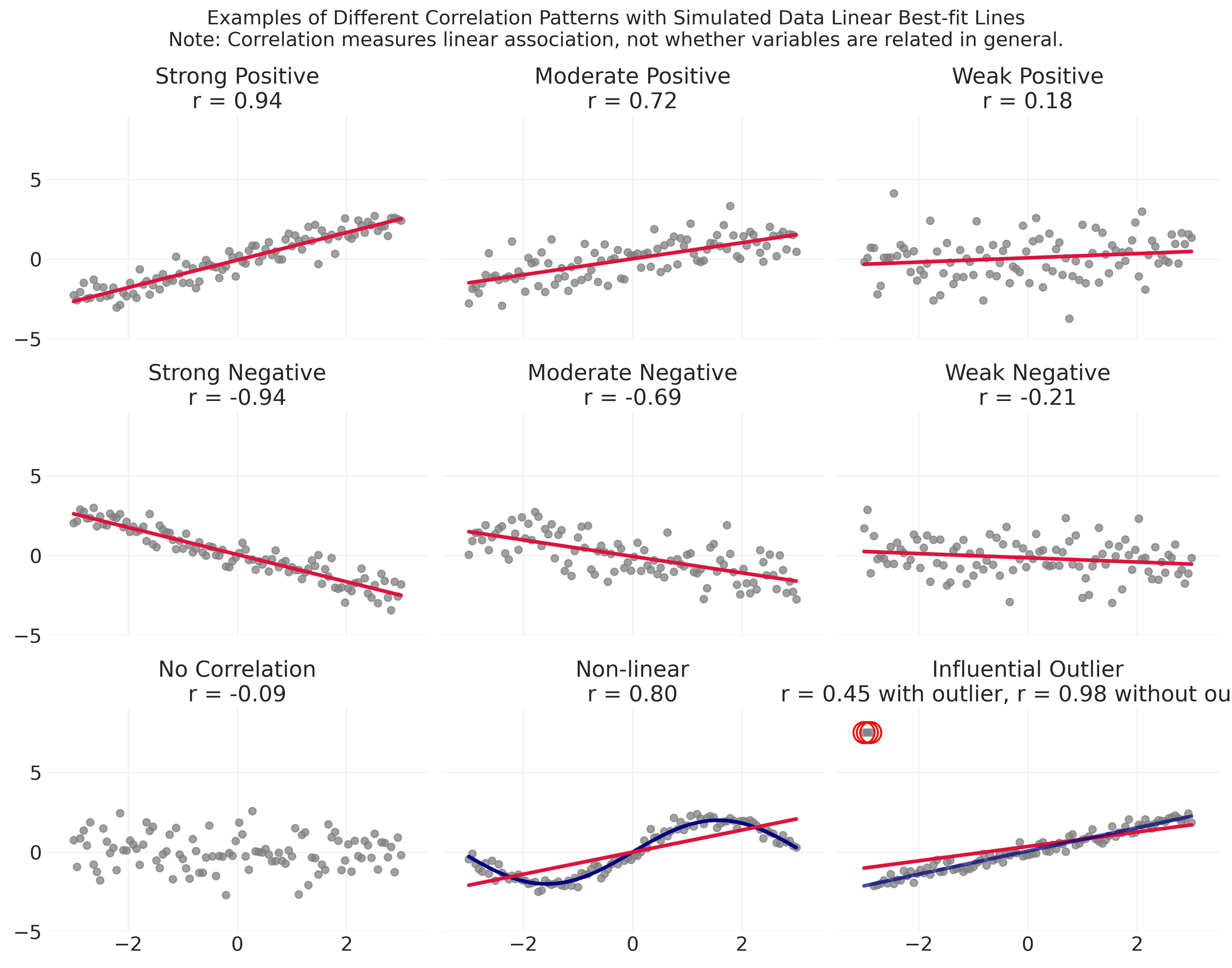
The bottom row illustrates a few additional things that are important to understand when working with correlations. First, when variables are truly unrelated, \(r\) hovers near zero and the scatterplot shows no obvious pattern.
Second, correlation can be misleading when relationships are non-linear. The middle panel shows a clear curved relationship (navy line), yet correlation only measures how well a straight line (crimson line) fits the data. The result is a moderately high \(r = 0.80\), even though the linear model completely misses the true pattern. This is one reason why you should always visualize relationships, especially when correlation coefficients seem surprisingly high or low.
Third, outliers can dramatically distort correlation, sometimes inflating it, sometimes suppressing it. The rightmost panel shows a strong positive linear relationship (navy line, \(r = 0.98\)), but three extreme outliers (circled in red) pull the correlation down to just \(r = 0.45\) (crimson line). Without checking the scatterplot, you might conclude there’s only a moderate association when the true relationship among most observations is actually quite strong.
Correlation coefficients are most meaningful when the relationship is approximately linear and there are no influential outliers driving (or masking) the association. These kinds of problems can go undetected without an accompanying visualization, so it’s a good idea to visualize the same relationships you correlate.
Common Mistakes with Correlation
Some errors that are common when you first start working with correlation:
Confusing correlation with causation: r = 0.70 means two variables move together, not that one causes the other.
Ignoring non-linearity: Correlation only measures linear association. Variables with strong curved relationships can show r ≈ 0.
Overlooking outliers: A few extreme points can dramatically inflate or suppress correlations.
Forgetting the range: Correlations are bounded [-1, +1]. An r = 0.30 might seem small but is often meaningful in social science where many factors influence outcomes.
Comparing correlations across different samples: A correlation of r = 0.50 in one dataset may reflect a different underlying relationship than r = 0.50 in another dataset with different variable distributions.
Always visualize your data before trusting summary statistics.
7.3.2 An Empirical Example
Let’s examine the correlation between two items. One asks whether “People who don’t get ahead should blame themselves, not the system” (pes21_blame), and another asks whether “Women seek to gain power by getting control over men” (pes21_hostile2):
r_pes21_blame_pes21_hostile2 = round(pes["pes21_blame"].corr(pes["pes21_hostile2"]), 3)

print(
    f"""
    r_pes21_blame and pes21_hostile2
    Pearson correlation: {r_pes21_blame_pes21_hostile2}
    """
)
The standard scatterplot approach faces a challenge with Likert data: since both variables take only discrete values (1-5), many respondents share identical combinations, creating severe overplotting. A naive scatterplot shows only 25 possible points (5×5 combinations) regardless of sample size, making it impossible to see the actual distribution of responses or the strength of the relationship.
Figure 7.3 shows the correlation using a heatmap, which displays the count of respondents for each combination of responses:
# Create counts for each combination
plot_data = pes[["pes21_blame", "pes21_hostile2"]].dropna()
counts_matrix = pd.crosstab(
    plot_data["pes21_hostile2"], plot_data["pes21_blame"]
).reindex(index=range(1, 6), columns=range(1, 6), fill_value=0)

# Create the plot
fig, ax = plt.subplots(1, 1, figsize=(8, 6))
sns.heatmap(
    counts_matrix,
    annot=True,
    fmt=",d",
    cmap="Blues",
    cbar_kws={"label": "Count"},
    linewidths=1,
    linecolor="white",
    ax=ax,
)
ax.set_xlabel(
    "Blame for Not Getting Ahead\n"
    + r"$\longleftarrow$ Strongly disagree, Strongly agree $\longrightarrow$"
)
ax.set_ylabel(
    'Hostile Sexism: "Women seek to gain power..."\n'
    + r"$\longleftarrow$ Strongly disagree, Strongly agree $\longrightarrow$"
)
ax.set_title("r = 0.29\n")
ax.invert_yaxis()

plt.savefig("_figures/blame_vs_hostile2_scatter.png", dpi=300)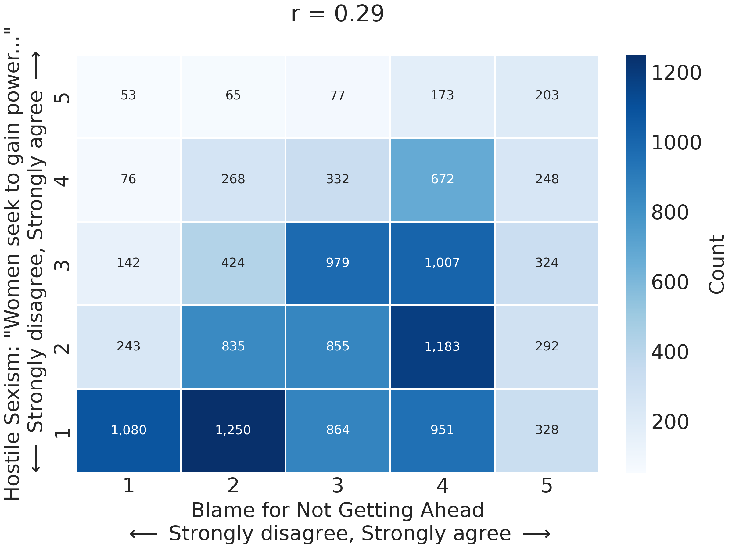
The heatmap reveals both the correlation and a key limitation of these data for illustrating association: the extreme skew in the hostile sexism variable means most respondents cluster at the lowest category (disagreeing with the hostile sexism item) regardless of their blame attitudes. This makes the positive correlation harder to see visually, even though it exists statistically (r = 0.29).
The modest positive correlation between these items suggests that respondents who endorse individualistic blame for lack of economic success tend to also endorse hostile sexist attitudes, though the relationship is far from deterministic. Most respondents (4,224 out of 12,103, or 35%) strongly reject the hostile sexism item (value = 1), and this concentration at the bottom of the distribution dominates the visualization. The positive association is visible in the subtle tendency for darker cells to appear along the diagonal from lower-left to upper-right, but this pattern is muted by the skewed marginal distribution.
7.3.3 Correlation Matrices
Rather than examining correlations one pair at a time, we can create a correlation matrix showing all pairwise correlations simultaneously. Let’s start with a small set and build up:
example_correlation_matrix = pes[
    [
        "pes21_blame",
        "pes21_hostile2",
        "pes21_hostile4",
        "pes21_famvalues",
        "pes21_hatespeech",
    ]
].corr()

example_correlation_matrix = round(example_correlation_matrix, 3)

example_correlation_matrix.to_markdown("_tables/example_correlation_matrix.md")
example_correlation_matrix| pes21_blame | pes21_hostile2 | pes21_hostile4 | pes21_famvalues | pes21_hatespeech | |
|---|---|---|---|---|---|
| pes21_blame | 1 | 0.287 | 0.358 | 0.365 | -0.106 |
| pes21_hostile2 | 0.287 | 1 | 0.66 | 0.359 | -0.178 |
| pes21_hostile4 | 0.358 | 0.66 | 1 | 0.369 | -0.21 |
| pes21_famvalues | 0.365 | 0.359 | 0.369 | 1 | -0.094 |
| pes21_hatespeech | -0.106 | -0.178 | -0.21 | -0.094 | 1 |
Notice how the diagonal in Table 7.8 is always 1.00 (every variable perfectly correlates with itself), and the matrix is symmetric (the correlation between A and B equals the correlation between B and A). We also see our first negative correlation: pes21_hatespeech (whether it should be illegal to say hateful things publicly) correlates negatively with the other items. This makes sense; the item about hate speech laws represents something different than the individual-blame, traditional-values, and hostile sexism captured by other items.
Now let’s examine all 45 attitude items at once:
# Ensure row/column names are variable names for clarity
likert_corr = pes[likert_cols].corr()

# Set row and column names to the explicit variable names for full clarity
likert_corr.index = likert_cols
likert_corr.columns = likert_cols

# Create a mask for the diagonal (True = hidden)
mask = np.eye(len(likert_corr), dtype=bool)

plt.figure(figsize=(16, 14))
sns.heatmap(
    likert_corr,
    mask=mask,
    annot=False,
    fmt=".2f",
    cmap="coolwarm",
    center=0,
    linewidths=1,
    cbar_kws={"shrink": 0.8, "label": "Correlation in the observed sample (r)"},
    xticklabels=likert_corr.columns,
    yticklabels=likert_corr.index,
)
plt.xlabel("")
plt.ylabel("")
plt.savefig("_figures/likert_heatmap.png", dpi=300)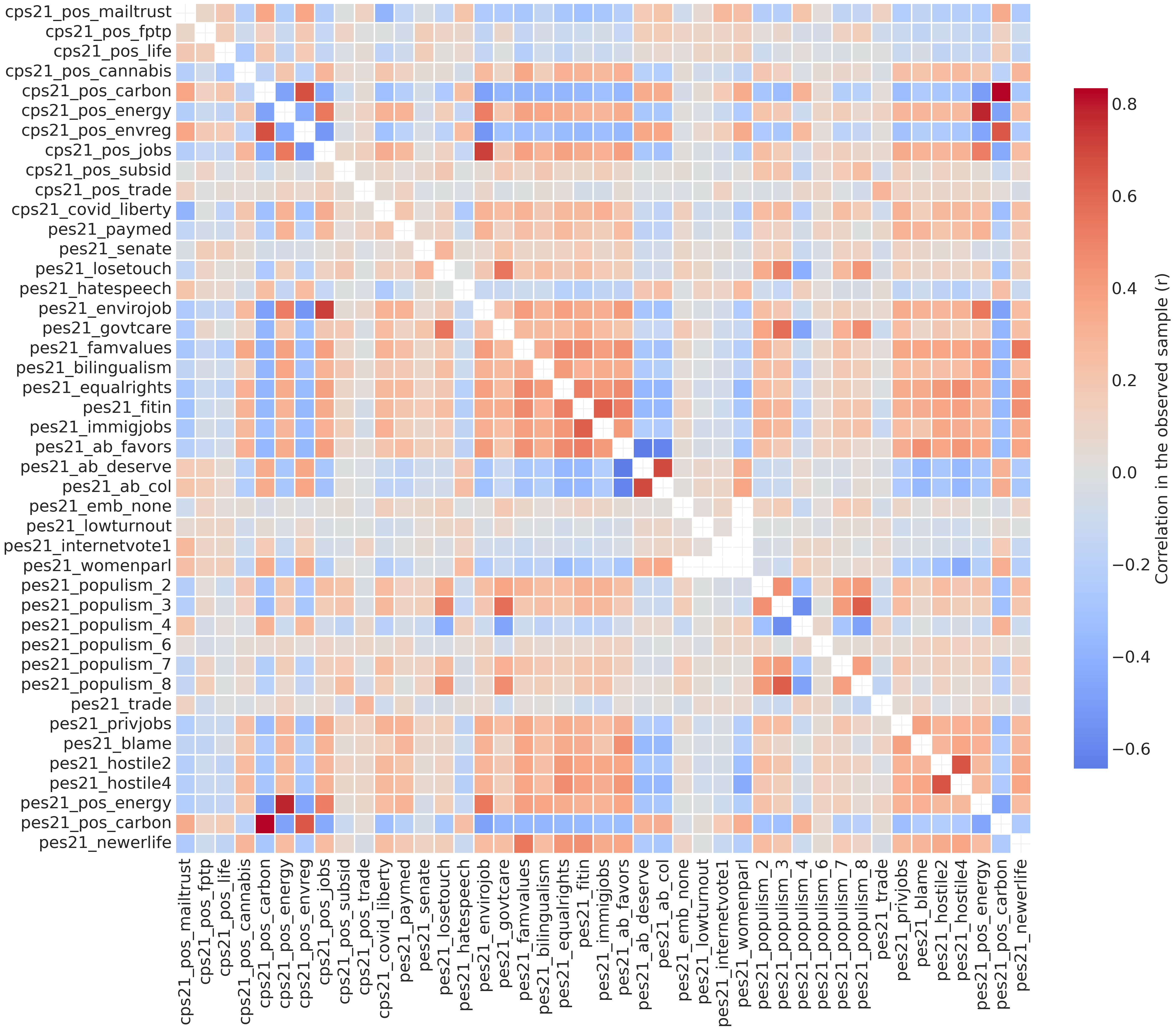
With 45 items, this correlation matrix contains 990 unique pairwise correlations (excluding the diagonal). The heatmap in Figure 7.4 reveals several patterns worth examining closely.
The CES 2021 survey uses the term “Aboriginal” in its question wording, reflecting terminology common at the time of data collection. Following current usage in Canada and preferences expressed by Indigenous communities, we use Indigenous when describing and interpreting results, while preserving the original survey wording when reporting question text for transparency and methodological accuracy.6
6 The CES 2021 survey uses the term “Aboriginal” in its question wording, reflecting terminology common at the time of data collection. Following current usage in Canada and preferences expressed by Indigenous communities, we use Indigenous when describing and interpreting results, while preserving the original survey wording when reporting question text for transparency and methodological accuracy.
7 Remember that in many cases, especially within-domain, these correlations are expected. They are by design in the sense that they are intended to be parallel manifest indicators of a shared latent construct.
First, we can see evidence of within-domain clustering. Several blocks of stronger correlations (darker red squares) appear where items on similar topics cluster together. The three Indigenous issues items (pes21_ab_favors, pes21_ab_deserve, pes21_ab_col) show strong correlations with each other, suggesting people who hold one view about Indigenous rights tend to hold consistent views across related questions.7 The two hostile sexism items (pes21_hostile2, pes21_hostile4) correlate very strongly (one of the darkest red cells in the entire matrix), indicating consistency in sexist attitudes. The populism items (pes21_populism_2 through pes21_populism_8) show moderate clustering, suggesting some internal structure for populist attitudes. Environmental items from both surveys (cps21_pos_carbon, cps21_pos_energy, cps21_pos_envreg, cps21_pos_jobs, pes21_envirojob, pes21_pos_carbon, pes21_pos_energy) also cluster, reflecting coherent positions on environment-versus-economy tradeoffs.
Second, it looks like there is cross-domain associations are weak. Despite within-domain clusters, the matrix is dominated by light orange and gray/white cells with a pattern indicating that correlations for items from different domains are generally weak. For example, attitudes about Indigenous issues don’t strongly predict attitudes about environmental policy or gender issues. This predominance of weak correlations suggests that overall attitude “constraint,” a concept we’ll discuss shortly, is relatively low in this sample.
Next we have the negative correlations, represented as blue cells scattered throughout the matrix. Carbon pricing attitudes (pes21_pos_carbon) negatively correlate with many other items, suggesting pro-environment positions run counter to populist, anti-immigrant, and traditional-values attitudes. The Indigenous reconciliation items also show negative correlations with some populist and traditional-values items, indicating an oppositional dimension between pro- and anti-Indigenous rights positions. Support for hate speech laws (pes21_hatespeech) also negatively correlates with several items, suggesting those who favour restricting hate speech tend to oppose traditional values and populist attitudes.
Taken together, these patterns suggest Canadian political attitudes are loosely structured. Respondents show strong consistency within specific issue domains (Indigenous rights, sexism, some populist themes) but weak connections across domains. Some oppositional dimensions exist (pro- vs. anti-environment, pro- vs. anti-Indigenous rights), but there’s no obvious, tightly integrated, left-right ideological structure linking all attitudes together.
This is consistent with a classic finding reported by Converse ([1964] 2006) in research on ideology and political belief systems in mass publics: most people don’t organize their beliefs into tightly integrated ideological systems. However, the within-domain clustering suggests people do develop coherent positions on specific issues, even if those positions don’t connect into a broader ideological framework.
To see this another way, we can plot the distribution of correlation coefficients. The result, shown in Figure 7.5, shows that most correlations are small and positive. The distribution’s mean captures the average level of constraint across all 990 issue pairs. Again, this suggests relatively low overall constraint: knowing someone’s position on one attitude provides only modest information about their positions on others (especially across issue domains, as we saw previously).
# Extract upper triangle values (excluding diagonal) and remove NaN
corr_distribution = likert_corr.values[np.triu_indices_from(likert_corr.values, k=1)]
corr_distribution = corr_distribution[~np.isnan(corr_distribution)]

plt.figure(figsize=(8, 5))
plt.hist(corr_distribution, bins=20, edgecolor="k", alpha=0.75, color="steelblue")
plt.xlabel("Correlation coefficient")
plt.ylabel("Frequency")

mean_corr = np.mean(corr_distribution)
plt.axvline(
    mean_corr,
    color="red",
    linestyle="--",
    linewidth=2,
    label=f"Mean: {mean_corr:.3f}",
)
plt.legend()
plt.tight_layout()
plt.savefig("_figures/distribution_of_correlation_coefficients.png", dpi=300)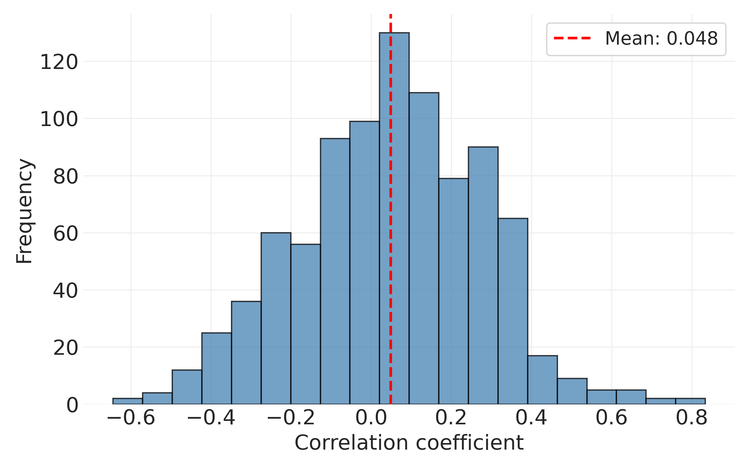
But this aggregate view obscures an important question about whether constraint varies across subgroups, for example different political groups.
7.3.4 Attitude Constraint by Partisan Identity
Advanced Section: Attitude Constraint
The following sections examine a sophisticated question in political psychology: how tightly are citizens’ political attitudes organized? This analysis is more advanced than earlier material but demonstrates real research in action.
Key concepts you’ll need:
- Correlation matrices (just covered)
- Comparing distributions across groups
- Distinguishing between average levels and structural patterns
If you find this section challenging, focus on the main finding: partisan groups differ in how tightly their attitudes connect, with implications for political representation. The technical details matter less than grasping that “constraint” refers to how much knowing one attitude helps predict others.
The aggregate patterns above reveal relatively low overall constraint, meaning that knowing someone’s position on one attitude provides limited information about their other positions. But this aggregate view raises an important question: does constraint vary across population subgroups, such as different political groups?
To answer this, we shift our analytical approach from calculating correlations for the entire sample to comparing correlation patterns across partisan identity subgroups. By examining how tightly attitudes connect within each partisan group, we can assess whether some groups organize their beliefs into more coherent systems than others. This comparative approach lets us move beyond describing average constraint levels to understanding how belief system structure varies across the political landscape.
Following Baldassarri and Gelman (2008), we can distinguish between two types of constraint:
- Issue Alignment: The correlation between pairs of issues (e.g., how well does your position on immigration predict your position on environmental policy?)
- Issue Partisanship: The correlation between party identification and issue positions (e.g., how well does knowing someone’s party predict their issue positions?)
Baldassarri and Gelman’s key finding was that over time (1972-2004), issue partisanship increased substantially while issue alignment remained stable. This means political parties became better at “sorting” voters along ideological lines, but individuals’ belief systems didn’t become more internally coherent. The polarization was driven by partisan sorting, not by citizens holding more tightly integrated belief systems.
However, as DellaPosta (2020) demonstrates, focusing only on mean correlations can obscure important structural differences. By focusing on explicitly “political” items, we may miss broader patterns of cultural and lifestyle alignment. Moreover, groups with identical average correlations could have fundamentally different belief network structures: which attitudes connect to which others, whether beliefs cluster into domains, and whether some beliefs serve as organizing “hubs.”
Below we examine both issue alignment and issue partisanship, and we look beyond simple means to examine the full distribution of correlations: their spread, range, and shape across partisan groups.
# Calculate both issue alignment and issue partisanship for each group
partisan_corr_distributions = {}  # Issue alignment (issue-to-issue)
issue_partisanship = {}  # Issue partisanship (party-to-issue)
respondent_counts = {}

for pid_code, pid_label in partisan_identity_mapping.items():
    # Filter data for this partisan identity
    pid_subset = pes[pes["pes21_pidtrad"] == pid_code]

    # Skip if too few observations
    if len(pid_subset) < 10:
        continue

    # === ISSUE ALIGNMENT: Correlation between pairs of issues ===
    corr_matrix = pid_subset[likert_cols].corr()

    # Extract upper triangle (excluding diagonal) and remove NaN
    corr_dist = corr_matrix.values[np.triu_indices_from(corr_matrix.values, k=1)]
    corr_dist = corr_dist[~np.isnan(corr_dist)]

    # Only store if we have valid correlations
    if len(corr_dist) > 0:
        partisan_corr_distributions[pid_label] = corr_dist
        respondent_counts[pid_label] = len(pid_subset)

        # === ISSUE PARTISANSHIP: Correlation between party ID and each issue ===
        # Use vectorized correlation calculation
        party_indicator = (pes["pes21_pidtrad"] == pid_code).astype(int)
        issue_party_corrs = pes[likert_cols].corrwith(party_indicator)
        issue_partisanship[pid_label] = issue_party_corrs.dropna().values

# Calculate global mean across all correlations for reference
all_correlations = np.concatenate(list(partisan_corr_distributions.values()))
global_mean = np.mean(all_correlations)
global_sd = np.std(all_correlations)

# Determine shared y-axis limit by getting max frequency across all groups
max_freq = 0
for corr_dist in partisan_corr_distributions.values():
    hist_vals, _ = np.histogram(corr_dist, bins=20, range=(-1, 1))
    max_freq = max(max_freq, hist_vals.max())
y_max = max_freq * 1.1  # Add 10% padding

# Create small multiples plot
fig, axes = plt.subplots(3, 3, figsize=(15, 12))
axes = axes.flatten()

for idx, (pid_label, corr_dist) in enumerate(partisan_corr_distributions.items()):
    ax = axes[idx]
    ax.hist(corr_dist, bins=20, edgecolor="k", alpha=0.75, color="steelblue")
    ax.set_xlabel("Correlation coefficient")
    ax.set_ylabel("Frequency")
    n_respondents = respondent_counts[pid_label]

    # Calculate statistics
    group_mean = np.mean(corr_dist)
    group_sd = np.std(corr_dist)

    ax.set_title(f"{pid_label} (N={n_respondents}, n={len(corr_dist)})")

    # Add group mean line
    ax.axvline(
        group_mean,
        color="red",
        linestyle="--",
        linewidth=2,
        label=f"Group: {group_mean:.2f}",
    )

    # Add global mean line for reference
    ax.axvline(
        global_mean,
        color="gray",
        linestyle=":",
        linewidth=2,
        label=f"Overall: {global_mean:.2f}",
    )

    # Add text box with SD
    textstr = f'SD: {group_sd:.3f}'
    ax.text(0.95, 0.70, textstr, transform=ax.transAxes, fontsize=8,
            verticalalignment='top', horizontalalignment='right',
            bbox=dict(boxstyle='round', facecolor='wheat', alpha=0.5))

    ax.legend(fontsize=8, loc="upper left")
    ax.set_xlim(-1, 1)
    ax.set_ylim(0, y_max)

# Hide any unused subplots
for idx in range(len(partisan_corr_distributions), len(axes)):
    axes[idx].axis("off")

plt.tight_layout()
plt.savefig("_figures/partisan_constraint_comparison.png", dpi=300)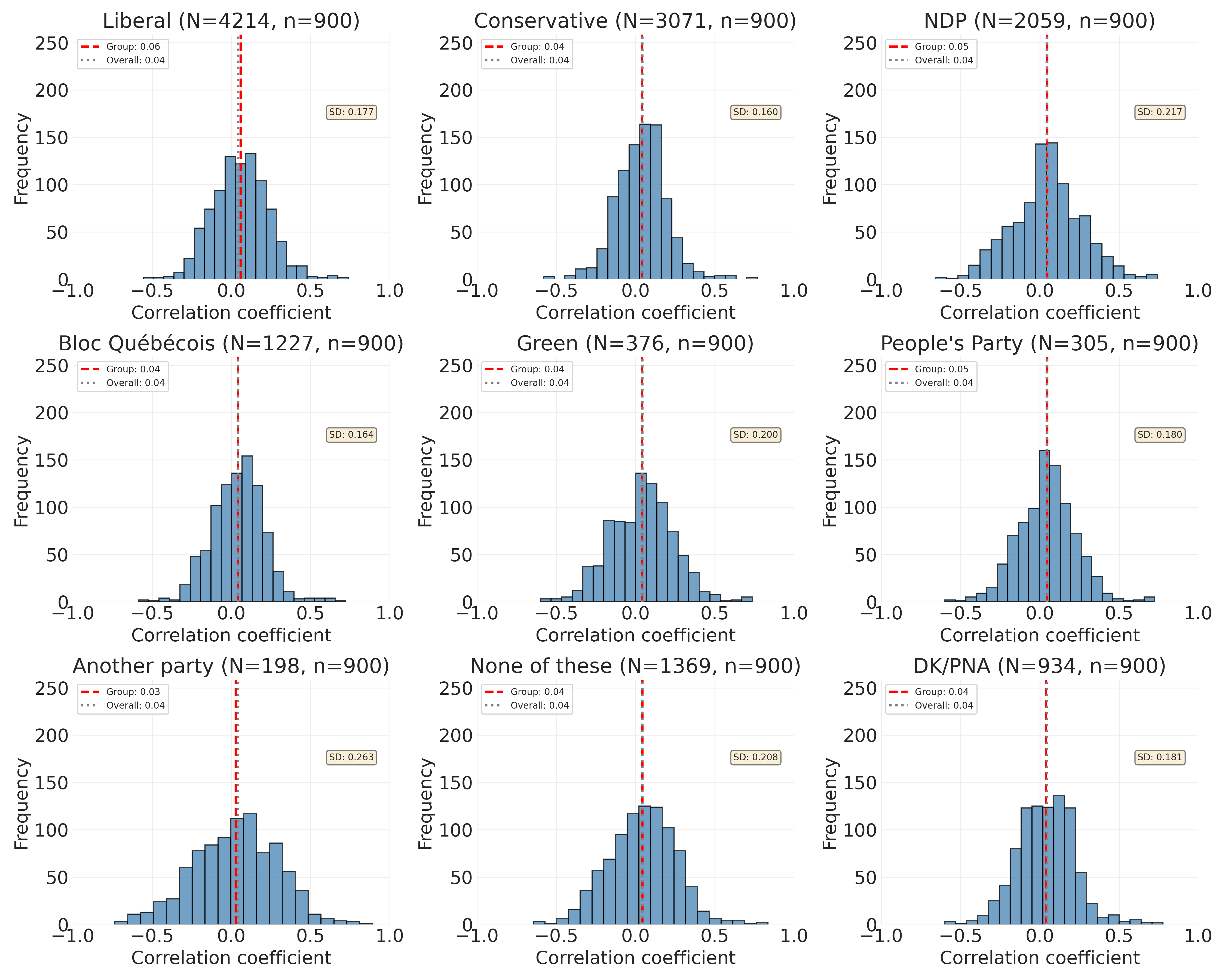
The patterns in Figure 7.6 reveal important differences in how political beliefs are organized across Canadian partisan groups. To understand these findings correctly, we must distinguish between two separate dimensions that are often confused in everyday language: extremity of positions and ideological coherence (constraint). The latter is focused only on the extent to which positions on different issues predict each other. If you know someone’s position on issue X, how well can you predict their position on issue Y? These dimensions are independent in the sense that you can be extreme without being coherent, or coherent without being extreme. Figure 7.6 measures the second dimension only, ideological coherence.
One thing you may notice in Figure 7.6 is that Liberals show the highest constraint (mean = 0.059), while the populist People’s Party shows middling constraint (mean = 0.046), and Conservatives show among the lowest constraint (mean = 0.041). This may seem counterintuitive if we assume that “more ideological” parties should have higher constraint. But this assumption conflates the two dimensions above.
Consider the People’s Party (PPC), often characterized as a far-right populist movement. If we interpret “ideological” to mean extreme positions, the PPC is indeed ideological—their supporters take distinctive positions on carbon pricing, immigration, and hate speech laws. However, Figure 7.6 shows that PPC supporters’ beliefs are not more tightly integrated across issues than Liberal supporters’ beliefs. In fact, they show less constraint.
This finding makes theoretical sense when we consider how populist parties form. Parties like the PPC are often protest coalitions or are defined primarily by a single-issue. Supporters may unite around specific grievances (opposition to carbon taxes, COVID-19 restrictions, and “political correctness”) without necessarily sharing a comprehensive worldview that organizes their positions across all political domains. Someone might support the PPC primarily for their stance on climate policy but hold views on other issues that don’t correlate strongly with that position.
In contrast, Liberals show the highest constraint. Liberal supporters’ beliefs form a more integrated package: knowing a Liberal’s position on economic inequality helps predict their positions on environmental policy, gender equality, Indigenous rights, and immigration. These issues are cognitively and ideologically linked for Liberal supporters in a way they are not for PPC supporters.
Conservatives, showing very low constraint (0.041), represent yet another pattern. Their low constraint likely reflects the Conservative Party’s big-tent coalition that accommodates diverse factions like fiscal conservatives, social conservatives, Western alienation populists, and Red Tories. These groups share party loyalty but may not share tightly correlated positions across all issues. This is the result of the several smaller parties merging under Stephen Harper, including the Canadian Alliance (Western populist-conservatives) and Progressive Conservative Party (traditional Red Tories) in 2003. This coalition, the Conservative Party of Canada, brought together fiscal conservatives, social conservatives, and Western alienation populists under one tent.
7.3.4.1 Constraint and Standard Deviation: Domain-Specific vs. Uniform Coherence
The standard deviations shown in each panel provide additional insight into belief system structure. Groups with higher standard deviations (like NDP at 0.217, “None of these” at 0.208, Green at 0.200) show domain-specific constraint: some pairs of issues are highly correlated while other pairs are weakly or even negatively correlated. This suggests beliefs organized into distinct modules or domains.
Groups with lower standard deviations (like Conservatives at 0.160, Bloc at 0.164, Liberals at 0.177) show more uniform patterns: correlations are more consistently moderate across all issue pairs, though still reflecting relatively loose overall organization.
“Another party” shows the most extreme pattern: the lowest mean (0.028) combined with the highest standard deviation (0.263) and widest range ([-0.73, 0.89]). This makes sense; it’s a heterogeneous catch-all category including supporters of various minor parties with radically different ideological projects, producing a chaotic mixture of strong positive, strong negative, and near-zero correlations.
7.3.4.2 Is This a “Non-Finding”?
Absolutely not. The modest levels of constraint across all parties (means ranging from 0.028 to 0.059) might seem like a non-finding if we expected much higher values. However, these results are substantively important for three reasons:
First, they confirm Converse’s classic finding ([1964] 2006) that most citizens do not organize their political beliefs into tightly integrated ideological systems. Even among partisan identifiers—the most politically engaged segment of the population—issue positions remain loosely connected. For Liberals, the group with highest constraint at a mean of 0.059, knowing someone’s position on one issue explains only about 0.35% of the variance in their position on another issue (r² = 0.059² ≈ 0.0035). The other 99.65% is unexplained. Most political cognition operates issue-by-issue rather than through abstract ideological frameworks.
Second, the differences across parties are modest but meaningful. In absolute terms, the differences are small—Liberal supporters show a mean correlation of 0.059 compared to 0.041 for Conservatives, a difference of only 0.018 correlation units. In terms of variance explained, Liberals’ issue positions share 0.35% common variance (r² = 0.059²) compared to 0.17% for Conservatives—a difference of just 0.18 percentage points.
However, these modest differences are meaningful in context. First, when the baseline is universally low (everyone below 0.06), any consistent pattern across 990 correlations suggests real structural differences in how beliefs are organized. Second, these patterns align with theoretical expectations about how different party types form coalitions. Third, Converse (1964) found mean correlations around 0.10-0.20 for ideologues and near zero for non-ideologues. Our range (0.028-0.059) suggests that by Converse’s standards, all Canadian partisan groups show relatively weak constraint, but with detectable variation in how much structure exists.
Third, these patterns have implications for democratic representation. Parties with lower constraint face a strategic challenge: their supporters don’t form neat ideological packages, making it difficult to represent them coherently. A party might take a strong position on issue X to satisfy one faction while that same faction holds diverse views on issue Y, Z, and W. This may explain why populist parties often resort to charismatic leadership and symbolic politics rather than comprehensive policy platforms—their supporters’ beliefs are organized around specific grievances rather than interconnected worldviews.
Table 7.9 presents the full statistical summary of both issue alignment and issue partisanship across all partisan groups, quantifying the patterns visible in Figure 7.6.
# Create comprehensive summary statistics table
summary_df = pd.DataFrame([
    {
        "Party": pid_label,
        "N": respondent_counts[pid_label],
        "Alignment Mean": np.mean(corr_dist),
        "Alignment SD": np.std(corr_dist),
        "Alignment Range": f"[{np.min(corr_dist):.2f}, {np.max(corr_dist):.2f}]",
        "Partisanship Mean": np.mean(np.abs(issue_partisanship[pid_label])),
        "Partisanship SD": np.std(np.abs(issue_partisanship[pid_label])),
    }
    for pid_label, corr_dist in partisan_corr_distributions.items()
]).sort_values("Alignment Mean", ascending=False)

# Format numeric columns
for col in ["Alignment Mean", "Alignment SD", "Partisanship Mean", "Partisanship SD"]:
    summary_df[col] = summary_df[col].apply(lambda x: f"{x:.3f}")

summary_df.to_markdown("_tables/constraint_summary_by_party.md", index=False)
summary_df| Party | N | Alignment Mean | Alignment SD | Alignment Range | Partisanship Mean | Partisanship SD |
|---|---|---|---|---|---|---|
| Liberal | 4214 | 0.059 | 0.177 | [-0.56, 0.74] | 0.132 | 0.073 |
| NDP | 2059 | 0.048 | 0.217 | [-0.66, 0.74] | 0.119 | 0.072 |
| People’s Party | 305 | 0.046 | 0.18 | [-0.60, 0.72] | 0.093 | 0.044 |
| None of these | 1369 | 0.044 | 0.208 | [-0.65, 0.84] | 0.04 | 0.036 |
| Bloc Québécois | 1227 | 0.042 | 0.164 | [-0.59, 0.72] | 0.064 | 0.054 |
| Green | 376 | 0.041 | 0.2 | [-0.60, 0.74] | 0.044 | 0.033 |
| Conservative | 3071 | 0.041 | 0.16 | [-0.58, 0.77] | 0.192 | 0.108 |
| DK/PNA | 934 | 0.04 | 0.181 | [-0.60, 0.78] | 0.02 | 0.015 |
| Another party | 198 | 0.028 | 0.263 | [-0.73, 0.89] | 0.024 | 0.014 |
Table 7.9 reveals several important patterns about belief system structure across partisan groups. Looking first at issue alignment (how issues correlate with each other within each group), we see means ranging from 0.028 to 0.059. These modest values suggest that across all parties, knowing someone’s position on one issue provides only limited information about their positions on other issues—consistent with Converse’s classic finding about weak constraint in mass publics.
However, the standard deviations tell a more nuanced story. Groups with higher SDs (like NDP at 0.217, “Another party” at 0.263) show more heterogeneous constraint: some issue pairs are highly correlated while others are weakly correlated, suggesting domain-specific belief organization. Groups with lower SDs (like Conservatives at 0.160, Bloc at 0.164) show more uniform constraint across all issue pairs. This variation in spread is invisible if we only examine means.
Looking at issue partisanship (how distinctively each group positions itself on issues), we see more meaningful differences. Conservatives show the strongest partisanship (0.192), meaning their members take highly distinctive positions that clearly differentiate them from other parties. Liberals (0.132) and NDP (0.119) also show moderately strong partisanship. Other groups show weaker partisanship (like Green at 0.044, “None of these” at 0.040, DK/PNA at 0.020), suggesting more overlap with other parties or more internal diversity. This pattern indicates that while Conservative supporters may have low issue alignment (weak correlations among their own attitudes), they nonetheless take distinctive collective positions that differentiate them sharply from other partisan groups.
The Importance of Examining Distributions, Not Just Means
The similar means (0.028-0.059) across parties obscure important structural differences visible in Figure 7.6. Consider the survey items: we now have 45 items spanning diverse domains including immigration (2), populism/political cynicism (7), Indigenous issues (3), gender equality/hostile sexism (3), environment/economy tradeoffs (7 items across both surveys), traditional values/social change (2), electoral and democratic institutions (4), healthcare (1), economic attitudes (4), and COVID-19 restrictions (1). Different partisan groups likely show constraint within specific issue domains rather than uniformly across all 45 items.
For example:
- People’s Party supporters might show high correlations among immigration attitudes and among anti-establishment attitudes, but these clusters might not correlate with each other or with other domains. This would produce a bimodal distribution with both high and low correlations.
- Green supporters might show tight correlations among environmental items and social issues, but weak correlations between these domains and economic policy, producing high variance.
- Liberal supporters might show more uniform moderate correlations across all domains, producing low variance but higher mean.
By averaging all 990 pairwise correlations together, we’re mixing within-domain correlations (potentially high, e.g., r = 0.70+ between related environmental items or hostile sexism items) with cross-domain correlations (potentially near zero or even negative). Groups with similar means could have fundamentally different distributions:
- High mean, low SD: Uniformly strong constraint across all issues (tightly integrated ideology)
- High mean, high SD: Strong constraint within domains, weak constraint between domains
- Low mean, low SD: Uniformly weak constraint (loosely organized beliefs)
- Low mean, high SD: Scattered pattern with some strong correlations mixed with weak/negative ones
The range values in Table 7.9 also matter: they show the extremes of the correlation distributions. For instance, “Another party” ranges from [-0.73, 0.89] while Conservatives range from [-0.58, 0.77] and Bloc ranges from [-0.59, 0.72]. These groups have fundamentally different belief structures despite having similar-looking mean correlations.
7.3.5 Constraint Across Other Subgroups
The partisan identity analysis revealed modest but meaningful variation in constraint. Do similar patterns emerge across other subgroups? Do older citizens show higher constraint than younger ones? Do more educated respondents organize beliefs more coherently?
These questions extend beyond our current scope but suggest important extensions. In applied research, you might examine constraint across:
- Political sophistication: Following Converse, more politically engaged citizens should show higher constraint
- Ideological self-placement: Self-identified ideologues may show tighter belief organization
- Age cohorts: Life experience and political socialization may affect constraint
- Education levels: Formal education might promote more integrated worldviews
7.4 Summary
This chapter introduced the logic of association, that is understanding how variables relate to and predict one another. We built progressively from simple descriptive tables to sophisticated analyses of belief system structure.
Categorical Association: We began with contingency tables and heatmaps, examining how attitudes toward income inequality differ across partisan identities. These tools revealed clear patterns: knowing someone’s partisan identity helps predict their views on economic inequality, with NDP and Green supporters much more likely than Conservatives to see inequality as a major problem. We learned to interpret joint distributions, marginal distributions, and conditional distributions—concepts that extend far beyond this single example.
Correlation for Numeric Data: We then turned to Pearson’s correlation coefficient (r) as a measure of linear association between numeric or quasi-numeric variables. Using 45 Likert-scale attitude items spanning environmental policy, immigration, Indigenous rights, gender equality, populism, and traditional values, we explored how political beliefs connect to one another. The overall pattern showed modest constraint, meaning Canadian respondents’ attitudes across different issues are weakly connected—a finding consistent with classic political science research on mass publics.
Distributions Matter More Than Means: When we compared constraint across partisan groups, we distinguished between issue alignment (correlations between pairs of issues) and issue partisanship (correlations between party identification and issue positions). While all groups showed modest mean alignment (0.028-0.059), the spread of correlation distributions revealed important structural differences. Groups with high standard deviations show domain-specific constraint (strong correlations within issue domains, weak correlations across domains). Groups with low standard deviations show more uniform patterns. Two groups with identical means can have fundamentally different belief structures—which attitudes connect to which others, which beliefs serve as organizing principles, and whether attitudes cluster into distinct domains or form an integrated whole.
Methodological Lessons: Throughout this chapter we encountered important methodological considerations:
- Contingency tables require careful attention to whether we’re showing row percentages, column percentages, or cell percentages
- Correlation measures only linear association and can be misleading with non-linear patterns
- Outliers can dramatically inflate or suppress correlations
- Visualization is essential—never trust summary statistics without examining the underlying distributions
- Likert-scale data occupies a pragmatic middle ground between ordinal and interval measurement
Looking Ahead: Association is foundational, but it cannot answer causal questions or account for confounding. In the next chapters, we’ll extend these ideas to measurement and regression, which allows us to examine multiple associations simultaneously and begin modeling the data-generating process more explicitly.